Download

1 / 42
420 likes | 587 Views
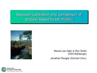
Bayesian calibration and uncertainty analysis of dynamic forest models. Marcel van Oijen CEH-Edinburgh. Input to forest models and output. Imperfect input data. Height. Environmental scenarios. NPP. Initial values. Soil C. Parameters. Model. Input to forest models and output. Model.

E N D
Bayesian calibration and uncertainty analysis of dynamic forest models Marcel van Oijen CEH-Edinburgh
Input to forest models and output Imperfect input data Height Environmental scenarios NPP Initial values Soil C Parameters Model
Input to forest models and output Model [Levy et al, 2004]
Input to forest models and output bgc century hybrid NdepUE (kg C kg-1 N) [Levy et al, 2004]
Simpler models? Goal: Robust models, predicting forest growth over 100 years, with low uncertainty Effects that must be accounted for: N-deposition CO2 Temperature Rain Radiation Soil fertility Management, e.g. thinning ... Are simple, robust models possible? Typical model size: 50 - 311 parameters
Simple (semi-)empirical relationships • Lieth (1972, “Miami”-model): NPP = f(Temperature, Rain) • Monteith (1977): NPP = LUE * Intercepted light • Gifford (1980): NPP = NPP0 (1 + β Log([CO2]/[CO2]0) ) • Gifford (1994): NPP = 0.5 GPP • Temperature ~ Light intensity • Roberts & Zimmermann (1999): LAImax Rain • Beer’s Law: Fractional light interception = (1-e-k LAI) • West, Brown, Enquist, Niklas (1997-2004): Height ~ Mass¼ ~ {fleaf, fstem, froot} • Brouwer (1983): Root-shoot ratio = f(N) • Goudriaan (1990): Turn-over rates, SOM,litter
BASic FORest model (BASFOR) BASFOR 39 parameters 24 output variables
BASFOR: Inputs Weather & soil: Skogaby (Sweden) BASFOR 24 output variables
Forest data from Skogaby (Sweden) Skogaby Planted: 1966, (2300 trees ha-1) Weather data: 1987-1995 Soil data: C, N, Mineralisation rate Tree data: Biomass, NPP, Height, [N], LAI
BASFOR: Inputs Weather & soil: Skogaby (Sweden) BASFOR 24 output variables
BASFOR: Inputs P(p1) p1,max p1,min Weather & soil: Skogaby (Sweden) BASFOR 24 output variables P(p39) p39,max p39,min
BASFOR: Prior predictive uncertainty Wood C Height NPP Skogaby, not calibrated (m ± σ)
BASFOR: Predictive uncertainty Calibration of parameters Data: measurements of output variables BASFOR 39 parameters High input uncertainty 24 output variables High output uncertainty
Calibration Bayesian calibration: P(p|D) = P(p) P(D|p) / P(D) P(p) L(f(p)|D) “Posterior distribution” “Prior distribution” Calibration = “Find P(p|D)” “Likelihood” given mismatch between model output & data: f P(p) P(f(p)) D
Calibration f P(p) P(f(p)) D Bayesian calibration P(p) P(f(p))
Data Skogaby (S) Wood C Height NPP
Calculating the posterior distribution Solutions Sampling problem: Markov Chain Monte Carlo (MCMC) methods Computing problem: Computer power, Numerical software Bayesian calibration: P(p|D)P(p) L(f(p)|D) • Calculating P(p|D)costs much time: • Sample parameter-space representatively • For each sampled set of parameter-values: • Calculate P(p) • Run the model • Calculate errors (model vs data), and their likelihood
Markov Chain Monte Carlo (MCMC) • Start anywhere in parameter-space: p1..39(i=0) • Randomly choose p(i+1) = p(i) + δ • IF: [ P(p(i+1)) L(f(p(i+1))) ] / • [ P(p(i)) L(f(p(i))) ] > Random[0,1] • THEN: accept P(i+1) & i=i+1 • ELSE: reject P(i+1) • 4. IF i < 104 GOTO 2 • E.g. {SLA=5, k=0.4, ... <39 parameters> ...} • Use multivariate normal distribution for [δ1, ... ,δ39] • Run BASFOR. • Assume normally distributed errors: L(output-dataj) ~ N(0,σj) with different σj for each datapoint MCMC: walk through parameter-space, such that the set of visited points approaches the posterior parameter distribution P(p|D) Metropolis algorithm BASFOR (~ 30 lines of code)
MCMC parameter trace plots: 10000 steps Param. value Steps in MCMC
Parameter correlations (PCC) 39 parameters 39 parameters
Posterior predictive uncertainty Skogaby, calibrated (m ± σ) Wood C NPP Height
Posterior predictive uncertainty vs prior Wood C NPP Height Skogaby, not calibrated (m ± σ) Skogaby, calibrated (m ± σ)
Partial correlations parameters – output variables 24 output variables Wood C 39 parameters
Partial correlations parameters – wood C Allocation to wood Senescence stem+br. Max Nleaf Nroot SOM turnover x p
Should we measure the “sensitive parameters”? • Yes, because the sensitive parameters: • are obviously important for prediction • No, because model parameters: • are model-specific • are correlated with each other, which we do not measure • cannot really be measured at all • So, it may be better to measure output variables, because they: • are what we are interested in • are better defined, in models and measurements • help determine parameter correlations if used in Bayesian calibration
The value of NPP-data Wood C NPP Height Skogaby, not calibrated (m ± σ) Skogaby, calibrated on NPP-data only (m ± σ)
Data of height growth: poor quality Wood C NPP Height Skogaby, not calibrated (m ± σ) Skogaby, calibrated on poor height-data only (m ± σ)
Data of height growth: high quality Skogaby, not calibrated (m ± σ) Skogaby, calibrated on poor height-data only (m ± σ) Skogaby, calibrated on good height-data only (m ± σ) Wood C NPP Height
Model application to forest growth in Rajec (Czechia) Skogaby Rajec (CZ): Planted: 1903, (6000 trees ha-1) Tree data: Wood-C, Height Rajec
Rajec (CZ): Uncalibrated and calibrated on Skogaby (S) Wood C NPP Height Rajec, not calibrated (m ± σ) Rajec, Skogaby-calibrated (m ± σ)
Rajec (CZ): Uncalibrated and calibrated on Skogaby (S) Wood C NPP Height Rajec, not calibrated (m ± σ) Rajec, Skogaby-calibrated (m ± σ)
Rajec (CZ): further calibration on Rajec-data Rajec, not calibrated (m ± σ) Rajec, Skogaby-calibrated (m ± σ) Rajec, Skogaby- and Rajec-calibrated (m ± σ) Wood C NPP Height
Summary of procedure “Error function” e.g. N(0, σ) MCMC Samples of f(p) (104 – 105) Samples of p (104 – 105) P(f(p)|D) PCC Posterior P(p|D) Prior P(p) Model f Data D ± σ Uncertainty analysis of model output Sensitivity analysis of model parameters Calibrated parameters, with covariances
Model selection Imperfect understanding Imperfect input data Imperfect output data Height Environmental scenarios NPP Initial values Soil C Parameters Model
Model selection Mean(log(L)) = -6.4 Mean(log(L)) = -8.7 Bayesian calibration: P(p|D)P(p) L(f(p)|D) Bayesian model selection: P(M|D)P(M) L(fM(pM)|D) Expolinear (4 parameters) BASFOR (39 parameters) Max(log(L)) = -5.7 Max(log(L)) = -6.9 “By-products” of MCMC
Conclusions (1) • Reducing parameter uncertainty: • Reduces predictive uncertainty • Reveals magnitude of errors in model structure • Benefits little from parameter measurement: • model parameter what you measure • parameter covariances are more important than variances • Requires calibration on measured outputs (eddy fluxes, C-inventories, height-measurement, ...) • Calibration: • Requires precise data • “Central” output variables are more useful than “peripheral” (NPP/gas exchange > height)
Conclusions (2) • MCMC-calibration • Works on all models • Conceptually simple, grounded in probability theory • Algorithmically simple (Metropolis) • Not fast (104 - 105 model runs) • Produces: • Sample from parameter pdf (means, variances and covariances), with likelihoods • Corresponding sample of model outputs (UA) • Partial correlation analysis of outputs vs parameters (SA) • Model selection • Can use the same probabilistic approach as calibration • Can use mean model log-likelihoods produced by MCMC
Acknowledgements • Göran Ågren (S) & Emil Klimo (CZ) • Peter Levy, Renate Wendler, Peter Millard (UK) • Ron Smith (UK)
MCMC: to do • Burn-in • Multiple chains • Mixing criteria (from characteristics of individual chains and from comparison of multiple chains) • Better (dynamic? f(prior?)) choice of step-length for generating candidate next points in p-space • Other speeding-up tricks?