Download
1 / 20
250 likes | 541 Views
2.4 Other Types of Equations. Objectives: Solve absolute-value equations. Solve radical equations. Solve fractional equations. Geometric Definition of Absolute Value. Take for instance the simple equation:

E N D
2.4 Other Types of Equations Objectives: Solve absolute-value equations. Solve radical equations. Solve fractional equations.
Geometric Definition of Absolute Value Take for instance the simple equation: Geometrically this is asking for what numbers on the number line have a distance from 0 of 4 units. The distance of a number from 0 on the number line. While 4 is the obvious answer, −4 is also a valid answer. Thus, there are two answers to this simple equation. 4 units 4 units
Example #1Using Absolute Value and Distance • Solve using the geometric definition. This problem can be thought of as the distance between x and 3 is 5 units. 5 units 5 units Therefore, there are two solutions to this equation, −2 & 8.
Algebraic Definition of Absolute Value Like the geometric definition, the algebraic definition specifies two possible answers. Therefore, when solving an absolute value equation algebraically, it is important to solve for both possibilities and then check for extraneous solutions or extraneous roots(“extra” solutions that do not make the original equation true). The algebraic definition is important because it allows us to solve equations that cannot be geometrically solved using a number line. If c ≥ 0, then If c < 0, then
Example #2Using the Algebraic Definition of Absolute Value Checking solutions: When both solutions are checked, one of the answers is shown to be extraneous.
Example #2Using the Algebraic Definition of Absolute Value The solution to this equation can also be checked graphically using the intersection method. Using this method we see that only one solution is valid.
Example #3Solving an Absolute Value Equation • Solve. When the degree of an absolute value equation is increased, so is the number of possible solutions. The example above has four possible solutions. A normal quadratic equation would only have two. Rather than checking by hand it may be faster to check with a graph.
Example #3Solving an Absolute Value Equation • Solve. From the intersection method and the graph, all four solutions can be seen and none are extraneous.
The Power Principle • Any equation that has both sides raised to the same positive integer power will keep every solution from the original. However, the new equation may also have extraneous solutions that were not part of the original problem. • Example of Power Principle: • When using the Power Principle keep in mind the following: • Only one radical may be removed at a time. • If after using it once a radical still remains, isolate the radical again and reapply it.
Example #4Solving a Radical Equation. • Solve. Isolate the radical first. Checking Solutions: By checking solutions we see that x = −2 is extraneous.
Example #4Solving a Radical Equation. • Solve. x = 4 is the only solution and x = −2 is extraneous. Graphing with the intercept method gives us:
Example #5Using the Power Principle Twice. • Solve. As before, isolate the radical first. Caution! does NOT simplify to it must first be expanded to
Example #5Using the Power Principle Twice. • Solve. As before we need to check for extraneous solutions, but we’ll do it by graphing and first show an alternative algebraic solution.
Example #5Using the Power Principle Twice. • Solve. As you can see both solutions take about the same time to find.
Example #5Using the Power Principle Twice. • Solve. The solution can also be verified graphically using the intercept method. x = 2 is the only solution as x = 14 is extraneous.
Example #6Distance Application • An industrial engineer is designing a conveyor belt system for a factory. An item will move a distance of d meters along the belt from point P to point Q and then drop onto another belt and move x meters from point Q to point R. He needs to position Q so that and item will get from P to R in 4 minutes 24 seconds. The belt from P to Q will move at the rate of 4 meters per minute and the belt from Q to R will move at the rate of 10 meters per minute. Find the required distance x from Q to R. P We start by finding d using the Pythagorean Theorem. d 8 m Q R 20 − x x 20 m
Example #6Distance Application Since distance equals rate times time, we can solve this for time and get an equation for the time it takes to travel from P to Q. P Total Time = (Time from P to Q) + (Time from Q to R). d 8 m Q R 20 − x x 20 m
Example #6Distance Application Finally we can set the equation equal to 0 and use the graphing calculator and the intercept method to solve for x. P There are two zeros for this function, 8.05 and 22.81. Only 8.05 m makes sense for this application so that is where Q should be placed. d 8 m Q R 20 − x x 20 m
Solving a Fractional Equation • When solving an equation of the form , the solution set includes all values of x such that f(x) = 0, so long as g(x) ≠ 0. Basically, this means that the equation can be solved simply by setting the numerator equal to 0, as long as once all solutions are found, they are checked to make sure the denominator doesn’t equal 0.
Example #7Solving a Fractional Equation. • Solve. Set the numerator equal to 0 and solve by factoring with Bottoms Up. Checking Solutions: The only solution is x = 1 since the other solution makes the denominator become 0.