Download
1 / 24
240 likes | 315 Views
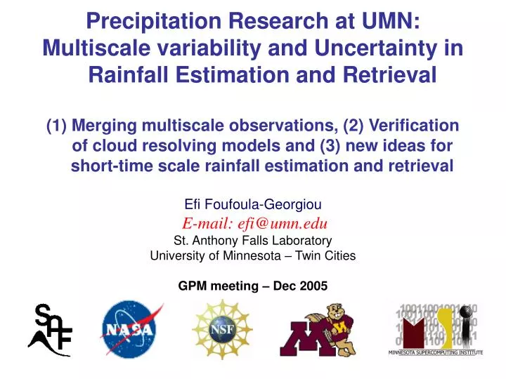
Precipitation Research at UMN: Multiscale variability and Uncertainty in Rainfall Estimation and Retrieval Merging multiscale observations, (2) Verification of cloud resolving models and (3) new ideas for short-time scale rainfall estimation and retrieval Efi Foufoula-Georgiou

E N D
Precipitation Research at UMN: • Multiscale variability and Uncertainty in Rainfall Estimation and Retrieval • Merging multiscale observations, (2) Verification of cloud resolving models and (3) new ideas for short-time scale rainfall estimation and retrieval • Efi Foufoula-Georgiou • E-mail: efi@umn.edu • St. Anthony Falls Laboratory • University of Minnesota – Twin Cities • GPM meeting – Dec 2005
THREE AREAS OF FOCUS • Developing nonparametric schemes for merging multisensor precipitation products Gupta, R., V. Venugopal and E. Foufoula-Georgiou, A methodology for merging multisensor precipitation estimates based on expectation-maximization and scale recursive estimation, in press, J. Geophysical Research, 2005. • 3D modeled cloud structure verification for satellite rainfall retrieval assessment Smedsmo, J., V. Venugopal, E. Foufoula-Georgiou, K. Droegmeier, and F. Kong, On the Vertical Structure of Modeled and Observed Clouds: Insights for Rainfall Retrieval and Microphysical Parameterization, in press, J. Applied Meteorology, 2005. • Fine-scale structure of rainfall in relation to simultaneous measurements of temperature and pressure Lashermes, B., E. Foufoula-Georgiou and S. Roux, Air pressure, temperature and rainfall: Insights from a joint multifractal analysis, AGU Fall Session, San Francisco, December 2005. -- add ref of Phys Letters -- Label 1,2,3
DEVELOPING NONPARAMETRIC SCHEMES FOR MERGING MULTISENSOR PRECIPITATION PRODUCTS • Issues: • Precipitation exhibits scale-dependent variability • Precipitation measurements are often available at different scales and have sensor-dependent observational uncertainties (e.g. raingauges, radars, and satellites) • It is not straightforward to optimally merge such measurements in order to obtain gridded estimates, and their estimation uncertainty, at any desired scale • Objective: • To develop a methodology that can: • handle disparate (in scale) measurement sources • account for observational uncertainty associated with each sensor • incorporate a multiscale model (theoretical or empirical) which captures the scale to scale characteristics of the process • Expected Result: • High quality merged/blended global precipitation estimates and their error statistics at different spatio-temporal scales
Fig. 1 Quadtree Representation of a Multiscale Process Satellite Scale 1 Radar Scale 2 Sparsely distributed measurements at the finer scale (gray dots), and measurements at a coarser scale (solid black dots), are placed on an inverted quadtree and merged via filtering and smoothing to obtain estimates at multiple scales Rainguage Network Scale 3
Scale Recursive Estimation (SRE) • measurement update • prediction at next coarser scale • merging of predictions • Consists of two steps • Upward Sweep (filtering) • Downward Sweep (smoothing) • Gives precipitation estimates at multiple scales + their variance (uncertainty) • Needs a multiscale model which relates the process from one scale to another m0 incorporation of neighborhood dependence m1 m2 Fig. 2 State-space equation: relates the process state from one scale to another W(λ) ~ N(0,1) Measurement equation: relates process measurements and state The parameter set of the multiscale state-space model is A(), B() , C(), R() | T, T is the set of all nodes in the tree
Estimation of Parameter B(λ) • Parametric Approach: MultiplicativeCascade models X() = X() W() Zero intermittency observed in precipitation presents a problem • Non-Parametric Approach: Variance Reduction Curves (VRC): Empirical variance as a function of scale (mm/hr) Sparsity of high-resolution data makes it difficult to estimate VRC Scale (km) Fig. 3 Proposed solution An approach based onExpectation Maximization which does not assume any apriori model prescribing multiscale variability, but rather uses the observations at multiple scales to dynamically evolve and simultaneously identify the parameters of the state-space equation (i.e., B()).
EM algorithm-based system identification • EM algorithm is used to iteratively solve for the Maximum Likelihood (ML) estimates of the parameters of the multiscale state-space equation. • Each iteration of the EM algorithm consists of two steps: • Expectation Step (E-Step) – uses Rauch-Tung-Striebel (RTS) algorithm to estimate the state of the process • Maximization Step (M-Step) – this step re-estimates the parameters using these uncertain state estimates • Main advantages of EM approach to SRE • No need for an a priori state-space model • No need to work in log-space • Scale-to-scale covariance explicitly used in model identification • Observational uncertainty explicitly used in model identification
Illustration of the application of SRE-EM methodology for the purpose of blending multi-sensor precipitation estimates 2x2 km field 16x16 km field ESTIMATED SRE 4x4 km field Input: 2x2 km field + its uncertainty 16x16 km field + its uncertainty Output: 4x4 km field, along with its uncertainty. Fig. 4
Comparison of observed vs. estimated fields Actual Field at 4x4 km Estimated Field at 4x4 km = 1.96 = 5.03 = 1.96 = 5.84 • Visually, the estimated field compares well with the observed field. • Comparison of basic statistics (mean and standard deviation) shows that SRE-EM is effective in producing unbiased estimates. • Spatial correlation is also reproduced well. RMSE = 0.96 Bias ~ 0.00 Spatial Correlation – X direction Spatial Correlation – Y direction estimated observed Fig. 5
Combining SRE-EM with downscaling schemes to produce consistent space-time blended precipitation products To address the issue of merging infrequent fine-resolution observations with frequent coarse-resolution observations to produce a consistent/reliable (in space and time) product, we performed a numerical experiment simulating three scenarios: Case 1is an idealized (best) case wherein observations are available at all times (t = 1, 2 and 3hr) at the coarse (16km) and fine (2km) resolutions. Case 2 is a scenario in which high-resolution information (2km) is available only at t = 1hr and the coarse resolution (16km) fields are available at all times (t = 1,2,3 hr). We perform a simple renormalization to match the total depth of water, i.e., R2km(t=2) = R2km(t=1) * R16km(t=2 or 3hr) / R16km(t=1), to obtain the 2 km field at t = 2 (or 3) hr. Case 3is a scenario in which the available fields are the same as Case 2, except the low-resolution information (16km) at t = 2 and 3 hr is spatially downscaled to obtain a statistically consistent (moments, spatial correlation) fields at 2 km at t = 2, 3hr. In all cases, 16 and 2 km fields (at t = 1, 2 and 3 hr) are input to SRE to obtain 4km fields at the respective times and these fields, in turn, are accumulated to obtain the 3-hr 4km fields
Downscaling (Case 3) improves the quality of the blended product Case 1 “True” RMSE = 1.45 BIAS ~ 0.00 RMSE = 11.07 BIAS ~ 0.00 Without downscaling With downscaling Case 2 Case 3 RMSE = 5.37 BIAS ~ 0.00 Fig. 7
Summary • Scale-recursive estimation is an effective procedure to blend precipitation-related information from multiple sensors. • Proposed Expectation-Maximization methodology addresses some of the drawbacks relating to the identification of the underlying multiscale structure of rainfall. • Downscaling methodologies have the potential to be used in conjunction with merging procedures to obtain spatially and temporally “consistent” products. • Future research will explore ways in which the proposed approach can be combined with a space-time downscaling scheme and/or temporal evolution of precipitation at a few locations only, such that the blended product at a desired scale incorporates all the available information in a space-time dynamically consistent way.
Discussion (Fig. 7) • Case 1 being the “best” case of available information, shows the least RMSE. This often is not realistically possible (compare top left and top right images in Fig. 7). • Cases 2 and 3 (with the same amount of information) represent more realistic scenarios in terms of available observations. However, the way we handle the information at the coarse scale dictates how well one can estimate an intermediate-scale field. • In case 2, since such a simple renormalization does not take into account possibilities such as the “appearance” of cells (or, “disappearance”), the resulting 4km field is bound to be far from the “truth” (compare top left and bottom left images in Fig. 7) • In case 3, we use the large-scale information effectively through a spatial downscaling scheme to resolve the small-scale variability. The visual comparison (compare top left and bottom right images in Fig. 7) of the observed and estimated (as well as quantitative comparisons such as the RMSE) is encouraging, and points to the advantages of using a spatial downscaling scheme. • The spatial downscaling scheme used is based on our previous work, and its effectiveness is demonstrated separately in Fig. 8
Merging of infrequent high-resolution and frequent low-resolution precipitation observations Given:16 x16 km precipitation estimates every 1 hour (e.g., satellite) 2 x 2 km precipitation estimates every 6 hours (e.g., radar) t = 0 t = 1 t = 2 t = 3 t = 4 t = 5 t = 6 16x16 km 2x2 km time (hrs) Objective:3-hr precipitation estimates at an intermediate scale of 4 x 4 km along with their uncertainties t = 0 t = 1 t = 2 t = 3 t = 4 t = 5 t = 6 time (hrs) 4x4 km Fig. 6
Performance of the spatial downscaling scheme used in Case 3 16KM The spatial downscaling scheme, which takes advantage of the presence of simple self-similarity in rainfall fluctuations, requires only one scaling parameter to resolve the small-scale variability (2km) given the large-scale variability (16km). This parameter has been found (Perica and Foufoula-Georgiou, JGR-Atmos. 101(D3); 101(D21), 1996) to be dependent on the available potential energy in the atmosphere (CAPE), and thus provide a viable (and parsimonious) means of resolving small-scale variability. SPATIAL DOWNSCALING 2KM 2KM Observed Fig. 8
Quadtree Representation of a Multiscale Process coarse Gridded Representation Quadtree Representation filtering Satellite scale 4 1 2 smoothing radar 1 3 4 3 2 2 3 4 1 1 2 1 2 3 2 3 4 3 4 3 4 2 1 gauges 4 1 1 2 1 2 2 3 4 3 4 3 1 4 fine Sparsely distributed measurements at the finer scale (gray dots), and measurements at a coarser scale (solid black dots), are placed on an inverted quadtree and merged via filtering and smoothing to obtain estimates at multiple scales Fig. 2
SRE Formulation State-space equation: relates the process state from one scale to another W(λ) ~ N(0,1) Measurement equation: relates process measurements and state V(λ) ~ N(0,R(λ)) The parameter set of the multiscale state-space model is If both measurements and the state of the system represent precipitation intensity, we can assume ‘A’ and ‘C’ to be unity. Therefore,
Estimation of Parameter B(λ) • Parametric Approach: Multiplicative Cascade models X() = X() W() coarse • Log-normal cascade (LN): m() = 0 , Z ~ N(0,1) “Root Scale” It can be shown that: B() = m() = 1 • Bounded Log-normal cascade: Weights lognormally distributed, but is chosen as a function of scale, : • bc() = 12-(m( )-1)H • 1bc(m() = 1) and H controls the decay rate of the variance Scale m() = 2 It can be shown that: B(λ) = bc(λ) fine Fig. 4 Zero intermittency observed in precipitation presents a problem
EM algorithm – Flow Chart Choose an initial parameter set θk :- K=0 E-Step: Estimate state using observations and parameter set θk Terminology: K = EM algorithm iteration Lk = Log-likelihood function ε= Tolerance θ = Parameter set {A(λ), B(λ), C(λ), R(λ)} M-Step: Compute maximum log-likelihood Lk+1 estimate of new parameter set θk+1 using estimated state K = K+1 Check for convergence??? (| Lk+1- Lk|< ε) See Appendix for details Fig. 6
APPENDIX: Details of EM algorithm • Log-likelihood function L(X,Yo,θ) is given as follows • The computation of log-likelihood function depends on three expectations • Kannan, A.et. al., “ML Parameter Estimation of a Multiscale Stochastic Process Using the EM Algorithm”, IEEE Trans. Signal Processing, Vol. 48, No. 6, 2000. • M. R. Luettgen and A. S. Willsky, “Multiscale Smoothing Error Models”, IEEE Trans. Automatic Control, Vol. 40, No. 1, 1995.
where The Expectation Step (E-step) • The E-Step of the algorithm computes the expected quantities required in the M-Step of EM algorithm • The terms and are computed by the downward sweep of the RTS algorithm • remains to be computed
is computed directly in the downward sweep by using the result that the smoothed error is a Gauss-Markov process has been shown to be modeled as a multiscale process of the following form The smoothed error is zero mean and white noise with covariance given by Computation of Luettgen, M. R., and Willsky, A. S., “Multiscale Smoothing Error Models” IEEE Trans. Automatic Control, Vol. 40, No. 1, 1995.
The Maximization Step (M-step) • This step maximizing the expected likelihood using multivariate regression to obtain new estimates of the parameters