Download
1 / 33
390 likes | 843 Views
Signal Detection Theory. March 25, 2010. Phonetics Fun, Ltd. Check it out: http://sakurakoshimizu.blogspot.com/. Another Brick in the Wall. Another interesting finding which has been used to argue for the “speech is special” theory is duplex perception . Take an isolated F3 transition:.

E N D
Signal Detection Theory March 25, 2010
Phonetics Fun, Ltd. • Check it out: • http://sakurakoshimizu.blogspot.com/
Another Brick in the Wall • Another interesting finding which has been used to argue for the “speech is special” theory is duplex perception. • Take an isolated F3 transition: and present it to one ear…
Do the Edges First! • While presenting this spectral frame to the other ear:
Two Birds with One Spectrogram • The resulting combo is perceived in duplex fashion: • One ear hears the F3 “chirp”; • The other ear hears the combined stimulus as “da”.
Duplex Interpretation • Check out the spectrograms in Praat. • Mann and Liberman (1983) found: • Discrimination of the F3 chirps is gradient when they’re in isolation… • but categorical when combined with the spectral frame. • (Compare with the F3 discrimination experiment with Japanese and American listeners) • Interpretation: the “special” speech processor puts the two pieces of the spectrogram together.
Some Psychometrics! • Response data from a perception experiment is usually organized in the form of a confusion matrix. • Data from Peterson & Barney (1952) • Each row corresponds to the stimulus category • Each column corresponds to the response category
Detection • In a detection task (as opposed to an identification task), listeners are asked to determine whether or not a signal was present in a stimulus. • For example--do the following clips contain release bursts? • Potential response categories: • SignalResponse • Hit: Present (in stimulus) “Present” • Miss: Present “Absent” • False Alarm: Absent “Present” • Correct Rejection: Absent “Absent”
Confusion, Simplified • For a detection task, the confusion matrix boils down to just two stimulus types and response options… • (Response Options) • PresentAbsent • Present Hit Miss • Absent False Alarm Correct Rejection (Stim Types) • Notice that a bias towards “present” responses will increase totals of both hits and false alarms. • Likewise, a bias towards “absent” responses will increase the number of both misses and correct rejections.
Canned Examples • From the text: in session 1, listeners are rewarded for “hits”. The resultant confusion matrix looks like this: • Present Absent • Present 82 18 • Absent 46 54 • The “correct” responses (in bold) = 82 + 54 = 136
Canned Examples • In session 2, the listeners are rewarded for “correct rejections”… • Present Absent • Present 55 45 • Absent 19 81 • The “correct” responses (in bold) = 55+ 81 = 136 • Moral of the story: simply counting the number of “correct responses” does not satisfactorily tell you what the listener is doing… • And response bias is not determined by what they can or cannot perceive in the signal.
Detection Theory • Signal Detection Theory: a “parametric” model that predicts when and why listeners respond with each of the four different response types in a detection task. • “Parametric” = response proportions are derived from underlying parameters • Assumption #1: listeners base response decisions on the amount of evidence they perceive in the stimulus for the presence of a signal. • Evidence = gradient variable. perceptual evidence
The Criterion • Assumption #2: listeners respond positively when the amount of perceptual evidence exceeds some internal criterion measure. criterion () “absent” responses “present” responses perceptual evidence • evidence > criterion “present” response • evidence < criterion “absent” response
The Distribution • Assumption #3: the amount of perceived evidence for a particular stimulus varies randomly… • and the variation is distributed normally. Frequency perceptual evidence The categorization of a particular stimulus will vary between trials.
Normal Facts • The normal distribution is defined by two parameters: • mean (= “average”) () • standard deviation () • The mean = center point of values in the distribution • The standard deviation = “spread” of values around the mean in the distribution. standard deviation standard deviation
Comparisons • Assumption #4: responses to both “absent” and “present” stimuli in a detection task will be distributed normally. • Generally speaking: • the mean of the “present” distribution will be higher on the evidence scale than that of the “absent” distribution. • Assumption #5: both “absent” and “present” distributions will have the same standard deviation. • (This is the simplest version of the model.)
Interpretation correct rejections false alarms criterion misses hits Important: the criterion level is the same for both types of stimuli… …but the means of the two distributions differ
Sensitivity • The perceptual distance between the means of the distributions reflects the listener’s sensitivity to the distinction. • Q: How can we estimate this distance? • A: We measure the distance of the criterion from each mean. • In normal distributions, this distance: • determines the proportion of responses on either side of the criterion • This distance = the criterion’s “z-score”
Z-Scores Hits Misses • Example 1: criterion at the mean • Z-score = 0 • 50% hits, 50% misses
Z-Scores Hits Misses • Example 2: criterion one standard deviation below the mean • Z-score = -1 • 84.1% hits, 15.9% misses
Z-Scores Hits Misses • Note: P(Hits) = 1-P(Misses) • z(P(Hits)) = z(1-P(Misses)) = -z(P(Misses)) • In this case: z(84.1) = -z(15.9) = 1
D-Prime • D-prime (d’) is a measure of sensitivity. • = perceptual distance between the means of the “present” and “absent” distributions. • This perceptual distance is expressed in terms of z-scores. n s d’
D-Prime Hits n s d’ • d’ combines the z-score for the percentage of hits…
D-Prime Hits n s -z(P(FA)) z(P(H)) False Alarms • d’ combines the z-score for the percentage of hits… • with the z-score for the percentage of false alarms. • d’ = z(P(H)) - z(P(FA))
D-Prime Examples 1. Present Absent • Present 82 18 • Absent 46 54 • d’ = z(P(H)) - z(P(FA)) = z(.82) - z(.46) = .915 - (-.1) = 1.015 2. Present Absent • Present 55 45 • Absent 19 81 • d’ = z(P(H)) - z(P(FA)) = z(.55) - z(.19) = .125 - (-.878) = 1.003 • Note: there is no absolute meaning to the value of d-prime • Also: NORMSINV() is the Excel function that converts percentages to z-scores.
Near Zero Correction • Note: the z-score is undefined at 100% and 0%. • Fix: replace those scores with a minimal deviation from the limit (.5% or 99.5%) • Present Absent • Present 100 0 • Absent 72 28 • d’ = z(P(H)) - z(P(FA)) = z(.995) - z(.72) = 2.57 - .58 = 1.99
Calculating Bias • An unbiased criterion would fall halfway between the means of both distributions. • No bias: P (Hits) = P (Correct Rejections) u b • Bias: P (Hits) != P (Correct Rejections)
Calculating Bias • Bias = distance (in z-scores) between the ideal criterion and the actual criterion u b • Bias () = -1/2 * (z(P(H)) + z(P(FA)))
For Instance Let’s say: d’ = 2 z(P(FA)) = -1 z(P(H)) = 1 • An unbiased criterion would be one standard deviation from both means… • z(P(H)) = 1 P(H) = 84.1% • z(P(FA)) = -1 P(FA) = 15.9%
Wink Wink, Nudge Nudge Now let’s move the criterion over 1/2 a standard deviation… z(P(FA)) = -.5 z(P(H)) = 1.5 • z(P(H)) = 1.5 P(H) = 93.3% (cf. 84.1%) • z(P(FA)) = -.5 P(FA) = 30.9% (cf. 15.9%) • Bias () = -1/2 * (z(P(H)) + z(P(FA))) • = -1/2 * (1.5 + (-.5)) = -1/2 * (1) = -.5
Calculating Bias: Examples • 1. Present Absent • Present 82 18 • Absent 46 54 • = -1/2 * (z(P(H)) + z(P(FA)) = -1/2 * (z(.82) + z(.46)) = -1/2 * (.915 + (-.1)) = -.407 • 2. Present Absent • Present 55 45 • Absent 19 81 • = -1/2 * (z(P(H)) + z(P(FA)) = -1/2 * (z(.55) + z(.19)) = -1/2 * (.125 + (-.878)) = .376 • The higher the criterion is set, the more positive this number will be.
Same/Different Example • With some caveats, the signal detection paradigm can be applied to identification or discrimination tasks, as well. • AX Discrimination data (from the CP task): • Pair Same Different Pair Same Different • 1-1 96 2 1-3 73 25 • 3-3 90 8 • We can combine the same pairs (1-1 and 3-3) to form the necessary same/different confusion matrix: • Same Diff. • Same 186 10 • Diff. 73 25
Same/Different Example • Let’s assume: • Hits = Same responses to Same pairs • False Alarms = Diff. responses to Same pairs • Same Diff. Total %(Same) • Same 186 10 196 94.9% • Diff. 73 25 98 74.5% • z(P(H)) = z(94.9) = 1.635 • z(P(FA)) = z(74.5) = .659 • d’ = z(P(H)) - z(P(FA)) = 1.635 - .659 = .977 • = -1/2*(z(P(H)) + z(P(FA)) = -.5*(1.635 + .659) = -1.147