Download
1 / 18
180 likes | 359 Views
Roles for Data Assimilation in Studying Solar Flares and CMEs. Brian Welsch, Bill Abbett , and George Fisher, Space Sciences Laboratory, UC Berkeley. O nly 17 minutes to talk, so here’s a quick summary of background in modeling flare/CME processes!.

E N D
Roles for Data Assimilation in Studying Solar Flares and CMEs Brian Welsch, Bill Abbett, and George Fisher, Space Sciences Laboratory, UC Berkeley
Only 17 minutes to talk, so here’s a quick summary of background in modeling flare/CME processes! 1. Physically, flares / CMEs are driven by the electric currents in the coronal magnetic field, BC. 2. Observationally, measurements of (vector) BC are not generally available. 3. Practically, BC must therefore be modeled. Which data should be used as input? 4. Physically, coronal magnetic energy originates in the interior, then passes across the photosphere and chromosphere, and upward into the corona. 5. Observationally, photospheric fields can be measured. 6. Hence, many coronal magnetic models are therefore derived from or driven by photospheric boundary data. Examples: A. Non-linear force-free fields (NLFFFs), e.g., Wiegelmann, Thalmann, et al.; DeRosa et al., 2009. B. Time-dependent models, e.g., Abbett & Fisher 2010; Cheung & DeRosa, in prep
Sequences of independent, static models (e.g., NLFFF extrapolations) can underestimate coronal energy. • Evolutionary techniques used to estimate a static NLFFF typically involve relaxation. • Further, most NLFFF extrapolation methods do not preserve topology. • Exception: FLUX code (DeForest & Kankelborg 2007) • NLFFF models can therefore approximately satisfy FFF and boundary conditions, but have less energy than actual field. • Antiochos, Klimchuk, & DeVore, 1999 Hence, dynamic coronal models show the most promise for deterministic forecasting.
Dynamic models have been described using terms with imprecise meanings. One possible classification: • Post-buildup: study eruption dynamics without focus on development of eruptive state --- e.g., start with an unstable flux rope, and simulate disruption. (e.g., CCHM eruption generator; Torok & Kliem 2005). • Data – inspired: use idealization of observed physical processes to drive eruption, e.g., flux cancellation (e.g., Amari, Aly, Mikic, & Linker 2010) • Data – driven: Use photospheric observations to derive time-dependent boundary condition for the coronal field. (e.g., Abbett & Fisher 2010; Cheung & DeRosa, in prep.) • Data Assimilation: Incorporateadditional data (e.g., coronal field measurements) into a dynamical model within the model domain. Implication: While assimilative models are consistent with data input, they are capable of running independently of input!
Poloidal-toroidal decomposition (PTD) can be used to derive electric fields for driving coronal models. ^ ^ ^ ^ tB = x ( x tB z) + x tJz -cEPTD= x tBz +tJz cETOT= cEPTD + ψ B = x ( xB z) +xJz Bz= -h2B, 4πJz/c= h2J, h·Bh= h2(zB) • See Fisher et al. 2010 ^ ^ Left: the full vector field B in AR 8210. Right: the part of Bh due only to Jz.
Cheung & DeRosa ran a data-driven magnetofrictional model using tB; but also imposed an ad-hoc vorticity of ω= 1/4 turn per day. Top view Orange ∝ L-1∫j2 dl Lavender ∝ L-1(B/Bbase)(∫j2 dl) y side view x side view Problem: can’t model forces in “lift-offs” – this model is, in fact, static!
The RADMHD model (Abbett 2007) can model dynamics in the upper layers of the convection zone to corona in a single domain. LEFT: Magnetic field lines initiated from a set of points located in the model chromosphere. The grayscale intensity on the horizontal slice representing the photosphere denotes the magnitude of vertical velocity along this layer. RIGHT: Magnetic field lines initiated from equidistant points along a horizontal line positioned near the upper boundary of the model corona. The image illustrates how magnetic flux entrained in overturning flows and strong convective downdrafts can be pushed below the surface. The horizontal slice denotes the approximate position of the photosphere, and grayscale contours of vertically directed flows (dark shades indicate downflows, while light shades indicate upflows) are displayed along the slice. INSET IMAGES: A timeseries (over ~ 5 minutes) of the magnetic flux penetrating a small portion of the model photosphere. This sub-domain is centered on the location featured in the background image where magnetic flux is being advected below the surface.
Assuming photospheric evolution is ideal, cE = -u x B, so u derived from estimates of E can be used to drive RADMHD. Fsim≡ –∇·[ ρuu + (p + B2/8π) I – BB/4π + ∏] +ρg Fdata≡ ∂t(ρuest) ∂t(ρuest)|phot = ξ (Fdata)⊥ +(1 - ξ) (Fsim)⊥ + (Fsim)|| • Here, 0 < ξ< 1 represents a Kalman-like “confidence matrix” defined at each mesh element within the photospheric volume. • ξ= 1: forces perp. to B are determined entirely by the data. • ξ= 0: forces perp. to B are determined entirely by the radiative-MHD system – no observational forcing! • Parallel (hydrodynamic) forces are always evolved by the MHD system.
Unfortunately, while tB provides constrains E, it does not fully determine E– any ψcan be added to E. Faraday’s law only relates tB to the curl of E, not E itself; the gauge electric field ψis unconstrained by tB. Ohm’s law is one additional constraint. Doppler shifts provide another constraint: where Blos = 0, the Doppler velocity and transverse magnetic field determine a Doppler electric field, cEDopp = – (vDopp x Btrans) Key issue: only true where BLOS = 0 – i.e., polarity inversion lines (PILS).
Fisher et al. (2011) tested a method of incorporating Doppler electric fields into estimates of total E. Top row: The three components of the electric field E and the vertical Poyntingflux Sz from the MHD reference simulation of emerging magnetic flux in a turbulent convection zone. 2nd row: The inductive components of E and Szdetermined using the PTD method. 3rd row: E and Szderived by incorporating Doppler flows around PILs into the PTD solutions. Note the dramatic improvement in the estimate of Sz. 4th row: E and Szderived by incorporating only non-inductive FLCT derived flows into the PTD solutions. Note the poorer recovery of Ex, Eyand Szrelative to the case that included only Doppler flows. 5th row: E and Sz derived by including both Doppler flows and non-inductive FLCT flows into the PTD solutions. Note the good recovery of Ex, Ey, and Sz, and the reduction in artifacts in the low-field regions for Ey.
But there’s a problem with using HMI data for this technique: the convective blueshift! Because rising plasma is (1) brighter (it’s hotter), and (2) occupies more area, there’s an intensity-blueshift correlation (talk to P. Scherrer!) S. Couvidat: line center for HMI is derived from the median of Doppler velocities in the central 90% of the solar disk --- hence, this bias is present! Punchline: HMI Doppler shifts are not absolutely calibrated! (Helioseismology uses time evolution of Doppler shifts, doesn’t need calibration.) Line “bisector” From Dravins et al. (1981)
Because magnetic fields suppress convection, there are pseudo-redshifts in magnetized regions, as on these PILs. Here, an automated method (Welsch & Li 2008) identified PILs in AR 11117, color-coded by orbit-corrected Doppler shift.
Ideally, the change in LOS flux ΔΦLOS/Δt should equal twice the flux change ΔΦPIL/Δtfrom vertical flows transporting Bhacross the PIL (black dashed line). ΔΦPIL/Δt ΔΦLOS/Δt • NB: The analysis here applies only near disk center!
We can use this constraint to calibrate the bias in the velocity zero point, v0, in observed Doppler shifts! A bias velocity v0 implies := “magnetic length” of PIL • ButΔΦLOS/2 should match ΔΦPIL, so we can solve for v0: (Eqn. 3) NB: v0 should be the SAME for ALLPILs==> solve statistically!
In sample HMI Data, we solved for v0 using dozens of PILs from several successive magnetograms in AR 11117. • v0 ± σ = 266 ± 46 m/s Error bars on v0 were computed assuming uncertainties of ±20 G on BLOS, ±70G on Btrs, and ±20 m/s on vDopp. • v0 ± σ = 320 ± 44 m/s • v0 ± σ = 293 ± 41 m/s
The inferred offset velocity v0 can be used to correct Doppler shifts along PILs.
Conclusions • Until measurements of the vector magnetic field BC in the corona can be made (efforts are underway!), BC can only be modeled. • Static models (e.g., extrapolations) likely underestimate coronal energies. • Magnetofrictional models cannot model eruptions, since they do not realistically treat the momentum equation. • We have developed assimilative methods to: • Derive electric fields, or flows, from magnetogram sequences using PTD; • Drive the RADMHD model by imposing flows derived via PTD E fields; • Incorporate Doppler data into our E field estimates (“PTD +Doppler”); • Correct offsets in HMI Doppler velocities from convective blueshifts.
Challenges: Modeling High & Low • High: Investigate use of coronal field measurements, e.g., field strengths from radio observations. • “8th wave” treatment can handle ·B= 0 • But updating B in the hyperbolic MHD system implies waves! • Low: Develop treatment of subsurface B and v • How can we incorporate observed flux emergence into the model in a self-consistent manner? • Global scales: models need global magnetic context • RADMHD is being converted to spherical coordinates -- “first NaN” expected soon, if not already achieved! • Large simulations are computationally expensive = difficult to run in real time!