Warm-up
170 likes | 248 Views
Warm-up. Do the work on the slip of paper (handout). Homework questions. Section 3.2. Least squares regression lines. regression line. A regression line is a straight line that describes how a response variable (y) changes as an explanatory variable (x) changes.

Warm-up
E N D
Presentation Transcript
Warm-up • Do the work on the slip of paper (handout)
Section 3.2 Least squares regression lines
regression line • A regression line is a straight line that describes how a response variable (y) changes as an explanatory variable (x) changes. • You can use a regression line to predict the value of y for any value of x by substituting this x into the equation of the line.
Interpreting regression lines • (read as “y hat”) is the predicted value of the y for a given value of x • b is the slope, the predicted change in y when x increases by 1 unit • a is the y-intercept, the predicted response variable when the explanatory variable equals zero (x=0)
Influential Point • An observation is influential if removing it would markedly change the position of the regression line. • Points that are outliers in the x direction are often influential.
extrapolation • Extrapolation is the use of a regression line for prediction using values of the explanatory variable (x) outside the range of the data from which the line was calculated. This should be avoided, as it leads to incorrect conclusions. • See warm-up… • What if I told you that the x’s were supposed to represent months and that the y’s were supposed to represent lows in temperature? Are your predictions still correct?
residuals A residual is the difference between an observed value of the response variable and the value predicted by the regression line. That is… Residual = observed y – predicted y =
Residual plots A residual plot is a scatterplot that uses our explanatory variable as the x and the residuals as the y. We can use the residual plot to determine if a scatterplot has a linear fit.
Two important things • The residual plot should show no obvious pattern. • A curved pattern shows that the relationship is not linear. A straight line may not be the best model for such data. • Increasing (or decreasing) spread about the line as x increases indicates that prediction of y will be less accurate for larger x (for smaller x). • The residuals should be relatively small in size.A regression line in a model that fits the data well should come “close” to most of the points. That is, the residuals should be fairly small. How do we decide whether the residuals are “small enough”? We consider the size of a “typical” prediction error.
Example – fat gain Almost all of the residuals are between −0.7 and 0.7. For these individuals, the predicted fat gain from the least-squares line is within 0.7 kg of their actual fat gain during the study. That sounds pretty good. But the subjects gained only between 0.4 kg and 4.2 kg, so a prediction error of 0.7 kg is relatively large compared with the actual fat gain for an individual. The largest residual, 1.64, corresponds to a prediction error of 1.64 kg. This subject's actual fat gain was 3.8 kg, but the regression line predicted a fat gain of only 2.16 kg. That's a pretty large error, especially from the subject's perspective!
Something unusual • Residuals from the least squares regression line have an unusual property – the mean of the residuals is always zero. • Why does this make sense?
Least squares regression line • The least squares regression line (LSRL) is the straight line that minimizes the sum of the squares of the vertical distances of the observed points from the line. • All LSRL’s go through the point • The LSRL is with • slope and • y-intercept
Calculating the Lsrl • The mean and standard deviation for this example are calories and calories. For the 16 people studied, the mean and the standard deviation are kg and kg. The correlation is r = 00.7786. Find the equation of the LRSL. Show your work.
Coefficient of determination • The coefficient of determination is the fraction of the variation in one variable that is accounted for by the LSRL on the other variable. • on your calc… • This measures how well the regression was in explaining the response. • If it means that 73% of the variation in y is due to the straight line relationship between x and y.
Caution! • Correlation and regression must be interpreted with caution. Plot the data to be sure that the relationship is roughly linear and to detect outliers. Also, the correlation and regression line are nonresistant, often outliers in x will greatly influence the regression line. • Most of all, be careful not to conclude that there is a cause-and-effect relationship between two variables just because they are strongly linear. (Don’t mistake correlation with causation!)
Homework • Page 191 (35-42, 44-46)
