Don Tinkle
Phylogenetics in Ecology Phylogenetic Systematics = Cladistics Shared derived characteristics (synapomorphies) Monophyletic groups = Clades Monophyletic, Polyphyletic, Paraphyletic Sister groups, outgroups, rooting trees Identify ancestral states — polarize character state changes

Don Tinkle
E N D
Presentation Transcript
Phylogenetics in EcologyPhylogenetic Systematics = CladisticsShared derived characteristics (synapomorphies) Monophyletic groups = Clades Monophyletic, Polyphyletic, ParaphyleticSister groups, outgroups, rooting trees Identify ancestral states — polarize character state changes Vicariance Biogeography, Area CladogramsPhylogeny and the Modern Comparative MethodPhylogenetically Independent ContrastsEvolutionary EcomorphologyConvergence (homoplasy)
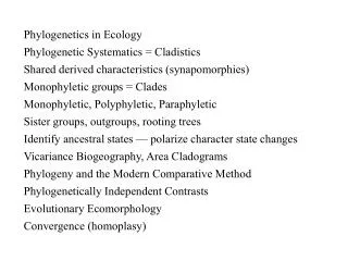
Jennings et al. 2003 Ophidiocephalus taeniatus Ophidiocephalus Pygopus Lialis Pygopus nigriceps Fossil Pygopus Lialis burtonis 22 myBP
Jennings and Pianka 2004 Bryan Jennings
Community and Ecosystem Ecology Macrodescriptors = Aggregate Variables Trophic structure, food webs, connectance rates of energy fixation and flow, ecological efficiency Diversity, stability, relative importance curves, guild structure, successional stages Communities are not designed by natural selection for smooth and efficient function, but are composed of many antagonists (need to attempt to understand them in terms of interactions between individual organisms)
Compartmentation Trophic Levels Autotrophs = producers Heterotrophs = consumers & decomposers Primary carnivores = secondary consumers Secondary carnivores = tertiary consumers Trophic continuum Horizontal versus vertical interactions Within and between trophic levels Guild Structure Foliage gleaning insectivorous birds Food Webs Subwebs, sink vs. source food webs Connectance
Compartment Models
Food Webs Bottom Line
Macrodescriptors = Aggregate VariablesTrophic structure, food webs, connectance Rates of energy fixation and flow, ecological efficiency Diversity, stability, relative importance curves Guild structure, successional stagesCommunities are not designed by natural selection for smooth and efficient function, but are composed of many antagonists (we need to attempt to understand them in terms of interactions between individual organisms – predator-prey coevolution) Systems Ecology, compartment models Compartmentation, Number of trophic levels, trophic continuum Autotrophs = producers Heterotrophs = consumers & decomposers Primary carnivores = secondary consumers Secondary carnivores = tertiary consumers
Biogeochemical cycles Horizontal versus vertical interactions (top-down, bottom-up) Trophic cascades Within and between trophic levels Guild structure, foliage gleaning insectivorous birds Food webs, subwebs, sink vs. source food webs, connectance Energetic importance of decomposers Ecological pyramids, pyramid of energy, inverted pyramids Standing crops versus rates of energy flow, Li, lij equations at equilibrium where dLdt = 0 for all i Ecological efficiency l32 / l21 average about 5-10% Gross productivity versus net productivity Secondary succession Horn’s transition matrix (a projection matrix)
Ecological Pyramids (numbers, biomass, and energy) Pyramid of energy Measures of standing crop versus rates of flow
Energy Flow and Ecological Energetics The energy content of a trophic level at any instant (i.e., its standing crop in energy) can be represented by capital lambda, L, with a subscript to indicate the appropriate trophic level: L1 = primary producers, L2 = herbivores, L3 = primary carnivores, and so on. Similarly, the rate of flow of energy between trophic levels is designated by lower case lambdas, lij , where the i and j subscripts indicate the two trophic levels involved with i representing the level receiving and j the level losing energy. Subscripts of zero denote the world external to the system; subscripts of 1, 2, 3, and so on, indicate trophic level as previously stated.
Energy Flow and Ecological Energetics At equilibrium (dLi/dt = 0 for all i), energy flow in the system portrayed in the figure may thus be represented by a set of simple equations (with inputs on the left and rate of outflow to the right of the equal signs): l10 = l01 + l02 + l03 + l04 l10 = l21 + l01 + l41 l21 = l32 + l02 + l42 l32 = l03 + l43 l41 + l42 + l43 = l04
Energy Flow and Ecological Energetics Gross Productivity Gross annual production (GAP) Net productivity Net annual production (NAP) Respiration in tropical rainforest 75-80% of GAP Respiration in temperate forests 50-75% of GAP In most other communities, it is 25-50 % of GAP Only about 5-10% of plant food is harvested by animals Remainder of NAP is consumed by decomposers
Transition Matrix for Institute Woods in Princeton _________________________________________________________________________ Canopy Sapling Species (%) Species BTA GB SF BG SG WO OK HI TU RM BE Total __________________________________________________________________________ BT Aspen 3 5 9 6 6 - 2 4 2 60 3 104 Gray birch - - 47 12 8 2 8 0 3 17 3 837 Sassafras 3 1 10 3 6 3 10 12 - 37 15 68 Blackgum 1 1 3 20 9 1 7 6 10 25 17 80 Sweetgum - - 16 0 31 0 7 7 5 27 7 662 White Oak - - 6 7 4 10 7 3 14 32 17 71 Red Oak - - 2 11 7 6 8 8 8 33 17 266 Hickory - - 1 3 1 3 13 4 9 49 17 223 Tuliptree - - 2 4 4 - 11 7 9 29 34 81 Red Maple - - 13 10 9 2 8 19 3 13 23 489 Beech - - - 2 1 1 1 1 8 6 80 405 __________________________________________________________________________ BTA in next generation = 0.03 BTA + 0.03 SF + 0.01 BG . Grand Total = 3286 Henry Horn
Distributions of Trees Observed in 4 Forests and Predicted Climax ____________________________________________________________________________________ Age (years) BTA GB SF BG SG WO OK HI TU RM BE ____________________________________________________________________________________ 25 0 49 2 7 18 0 3 0 0 20 1 65 26 6 0 45 0 0 12 1 4 6 0 150 - - 0 1 5 0 22 0 0 70 2 350 - - - 6 - 3 - 0 14 1 76 Predicted climax 0 0 2 3 4 2 4 6 6 10 63 ____________________________________________________________________________________ Data from the Institute Woods in Princeton (Horn 1975) Henry Horn