Download

1 / 31
310 likes | 500 Views
Using the Inner-Distance for Classification of Articulated Shapes. Haibin Ling and David Jacobs Center for Automation Research University of Maryland College Park. Problems: Three toys. Schedule. Related work The inner-distance and its properties

E N D
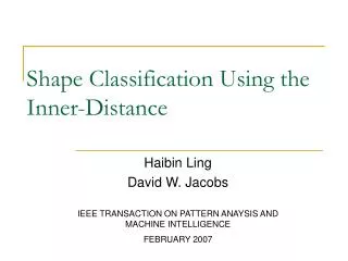
Using the Inner-Distance for Classification of Articulated Shapes Haibin Ling and David Jacobs Center for Automation Research University of Maryland College Park
Schedule • Related work • The inner-distance and its properties • Extension of shape context with the inner-distance • Silhouette matching using dynamic programming based on the new descripors • Experiment results
Related Works • Bending invariant signature for 3D surfaces, [Elad & Kimmel 2003]: geodesic distances + MDS • Shape context, [Belongie et al. 2002] • Two categories of methods for handling part structures: • Supervised methods explicitly build models for part structures through training. Grimson 1990, Felzenszwalb and Huttenlocher 2003, Schneiderman and Kanade 2004, etc. • Unsupervised methods: do not depend on explicit part models. Basri et al., Siddiqi&etal, Sebastian et al. 04, Gorelick et al., etc.
The Inner Distance • Given two points x, y in a shape O (O is a connected and closed subset of R2), the inner-distance between x,y, denoted as d(x,y;O), is defined as the length of the shortest path connecting x and y within O. • Reduced to the Euclidean distance for convex object. • Affected by concavity of shapes – a hint of part structure.
Properties of the Inner-Distance • Articulation Insensitivity • Articulation invariant for ideal articulated shapes • For most pairs of points in an articulated shape, the relative changes of their inner-distances are very small • Capturing part structures • Difficult to prove: the definition of part structure remains unclear • We show this with examples and analysis of experimental results
A Model of Articulated Shapes • Oi is a part; Jij is a junction between Oi, Oj • Oi and Oj has no common points • diameter(Jij) < ε, • The diameter is in the sense of the inner-distance • ε is very small compared to the parts. • When ε =0, all junctions degenerate to single points, O is called an ideal articulated object.
Articulations between Shapes • The articulation of shape O is a one-to-one mapping f fromO toO‘=f(O) • O' is also an articulated object, and decomposed to parts O’I and junctions J’ij where O'i=f(Oi), J'ij=f(Jij) . This preserves thetopology between the articulated parts. • f is rigid (rotation and translation only) when limited on each part. This means inner-distances within each part will not change.
Notations • f(P) denotes {f(x): x in P} • C(x1,x2;P) denotes a shortest path from x1 in P to x2 in P. (P is a closed and connected subset of R2. • ‘ indicates the image of a point or a point set under articulation f. • [ and ] denote the concatenation of paths.
Changes of Inner-Distance within Parts and Junctions • Fact 1: the inner-distance within any part is invariant to articulation • Fact 2: for two points in a same junction, the change of the inner-distance under articulation is bounded by ε
Articulation Insensitivity of the Inner-Distance Theorem: Let O be an articulated object and f be anarticulation of O as defined above. Let x,y be two arbitrary points in O. Suppose the shortest path C(x,y;O) goesthrough m different junctions in O and C(x',y';O') goesthrough m' different junctions in O', then |d(x,y;O)-d(x',y';O')| < max{m,m'}ε
Proof of the Articulation Insensitivity of the Inner-Distance • Decompose the shortest path C(x,y;O) into segments. Each segment is either within a part, or start and end in a same junction. • Construct a relaxed path in O’ according to the decomposition. • Apply the two facts mentioned above.
Illustration of the Proof • (a) Decomposition of C(x,y;O) with x=p0,p1,p2,p3=y. Note that a segment can go through a junction more than once (e.g. p1,p2). • (b) Construction of C”(x',y';O') in O'. Note that C”(x',y';O') is not the shortest path.
The Inner-Distance and Part Structure • The inner-distance captures part structures • With the same sample points, the distributions of Euclidean distances between all pair of points are virtually indistinguishable for the four shapes, while the distributions of the inner-distances are quite different
Another Interesting Case • With about the same number of sample points, the four shapes are virtually indistinguishable using Euclidean distances, while their distributions of the inner-distances are quite different except for the first two shapes. • 1) None of the shapes has (explicit) parts. • 2) More sample points will not affect much to the above statement.
Computing the Inner-Distance • Using shortest path algorithms • Build a graph on thesample points. For each pair of sample points x andy, if the linesegment connecting x and y falls entirely within the object,then build an edge between them with the weight equal tothe Euclidean distance |x-y|. • Apply a shortest pathalgorithm to the graph.
Application of the Inner-distance • Extend the shape context [Belongie 2002] for shape matching and comparison • Dynamic programming for silhouette matching • Other ways: • Multidimensional Scaling (MDS), Elad&Kimmel 2003 • Shape distribution [Osada et al. 2002]
Previous Work on Shape Context • Given n sample points x1,x2,...,xn on a shape, the shape context at point xi is defined as a histogram hi of the relative coordinates of the remaining n-1points [Belongie et al. 2002]: • [Belongie et al. 2002] proposed combining the shape context and thin-plate-spline (SC+TPS) for shape matching.
Extension to Shape Context --Inner-distance Shape Context (IDSC) • The Euclidean distance is directly replaced by the inner-distance. • The orientation between points is replaced by the inner-angle, which is defined as the angle between the tangential direction of the shortest path and the local tangential on the shape boundary.
The Inner-Angle • The inner-angle is insensitative to articulation.
Silhouette Matching through Dynamic Programming • Utilize the ordering provided by the contour. • Fast and accurate • Other works using dynamic programming: [Basri et al. 1998, Petrakis et al. 2002]. • Bipartite matching: more general, less constraint, slow.
Analysis of Experiment: MPEG7 Two retrieval examples for comparing SC and IDSC on the MPEG7 data set. The left column show two shapes to be retrieved: a beetle and an octopus. The four right rows show the top 1 to 9 matches, from top to bottom: SC and IDSC for the beetle, SC and IDSC for the octopus.
The Inner-Distance and Part Structure • We observed this data set is difficult for retrieval mainly due to thecomplex part structures in the shapes, though they have littlearticulation. This shows that the inner-distance iseffective at capturing part structures. • The following experiments also demonstrate similar effect.
Experiment: Swedish Leaf Dataset • Using 25 training samples and 50 testing samples per species. Average correct ratios are: • Combination of simple features: 82% [Soderkvist 2001] • Fourier descriptors: 89.60% • SC+DP: 88.12% • IDSC+DP: 94.13%
Experiment: Human Body Matching • Left: between adjacent frames. Right: silhouettes separated by 20 frames. Only half of the matched pairs are shown for illustration.