The Towers of Hanoi

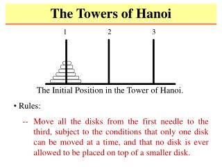
1. The Towers of Hanoi 1 2 3 • The Initial Position in the Tower of Hanoi. •  •Rules: • -- Move all the disks from the first needle to the third, subject to the conditions that only one disk can be moved at a time, and that no disk is ever allowed to be placed on top of a smaller disk.

2. The Idea • Begin with n disks on needle 1. We can transfer the top n - 1 disks, following the rules of the puzzle, to needle 3 using Hn-1 moves. We keep the largest disk fixed during these moves. Then, we use one move to transfer the largest disk to the second needle. We can transfer the n -1 disks on needle 3 to needle 2, using Hn-1 additional moves, placing them on top of the largest disk, which always stays fixed on the bottom of needle 2. Moreover, it is easy to see that the puzzle cannot be solved using fewer steps. This shows that Hn = 2Hn-1 + 1 • The initial condition is H1 = 1, since one disk can be transferred from needle 1 to needle 2.

3. The Algorithm Idea: move(63, 1, 2, 3); printf("Move a disk from needle 1 to needle 3.\n"); Move (63, 2, 3, 1); where Move(n, a, b, c); means move n desks from needle a to needle b using needle c as temporary storage.

4. The Implementation

5. Can’t Finish the Assigned Task “I can’t find an efficient algorithm, I guess I’m just too dumb.”

6. Mission Impossible “I can’t find an efficient algorithm, because no such algorithm is possible.”

7. 諾爾 愛斯坦 “I can’t find an efficient algorithm, but neither can all these famous people.”

8. Easy and Hard Problems • We argue that the class of problems that can be solved in polynomial time (denoted by P) corresponds well with what we can feasibly compute. But sometimes it is difficult to tell when a particular problem is in P or not. • Theoreticians spend a good deal of time trying to determine whether particular problems are in P. To demonstrate how difficult it can be. • To make this determination, we will survey a number of problems, some of which are known to be in P, and some of which we think are (probably) not in P. The difference between the two types of problem can be surprisingly small. Throughout the following, an ''easy'' problem is one that is solvable in polynomial time, while a ''hard'' problem is one that we think cannot be solved in polynomial time.

9. Eulerian Tour vs. Hamiltonian Tour • Eulerian Tours • INPUT: A graph G = (V, E). • DECIDE: Is there a path that crosses every edge exactly once and returns to its starting point? • Hamiltonian Tours • INPUT: A graph G = (V, E). • DECIDE: Is there a path that visits every vertex exactly once and returns to its starting point? -- Easy -- Hard

10. Some Facts • Eulerian Tours • A famous mathematical theorem comes to our rescue. If the graph is connected and every vertex has even degree, then the graph is guaranteed to have such a tour. The algorithm to find the tour is a little trickier, but still doable in polynomial time. • Hamiltonian Tours • No one knows how to solve this problem in polynomial time. The subtle distinction between visiting edges and visiting vertices changes an easy problem into a hard one.

11. Map Colorability • Map 2-colorability • INPUT: A graph G=(V, E). • DECIDE: Can this map be colored with 2 colors so that no two adjacent countries have the same color? • Map 3-colorability • INPUT: A graph G=(V, E). • DECIDE: Can this map be colored with 3 colors so that no two adjacent countries have the same color? • Map 4-colorability -- Easy -- Hard -- Easy

12. Some Facts • Map 2-colorability • To solve this problem, we simply color the first country arbitrarily. This forces the colors of neighboring countries to be the other color, which in turn forces the color of the countries neighboring those countries, and so on. If we reach a country which borders two countries of different color, we will know that the map cannot be two-colored; otherwise, we will produce a two coloring. So this problem is easily solvable in polynomial time.

13. Some Facts • Map 3-colorability • This problem seems very similar to the problem above, however, it turns out to be much harder. No one knows how this problem can be solved in polynomial time. (In fact this problem is NP-complete.) • Map 4-colorability. • Here we have an easy problem again. By a famous theorem, any map can be four-colored. It turns out that finding such a coloring is not that difficult either.

14. Problem vs. Problem Instance • When we say that a problem is hard, it means that some instances of the problem are hard. It does not mean that all problem instances are hard. • For example, the following problem instance is trivially 3-colorable:

15. Longest Path vs. Shortest Path • Longest Path • INPUT: A graph G = (V, E), two vertices u, v of V, and a weighting function on E. • OUTPUT: The longest path between u and v. • Shortest Path • INPUT: A graph G = (V, E), two vertices u, v of V, and a weighting function on E. • OUTPUT: The shortest path between u and v. -- Hard No one is able to come up with a polynomial time algorithm yet. -- Easy A greedy method will solve this problem easily.

16. Multiplication vs. Factoring • Multiplication • INPUT: Integers x,y. • OUTPUT: The product xy. • Factoring (Un-multiplying) • INPUT: An integer n. • OUTPUT: If n is not prime, output two integers x, y such that 1 < x, y < n and x  y = n. -- Easy -- Hard Again, the problem of factoring is not known to be in P. In this case, the hardness of a problem turns out to be useful. Some cryptographic algorithms depend on the assumption that factoring is hard to ensure that a code cannot be broken by a computer.

17. Boolean Formulas • Formula evaluation • INPUT: A boolean formula (e.g. (x y)  (z x)) and a value for all variables in the formula (e.g. x = 0, y = 1, z = 0). • DECIDE: The value of the formula. (e.g., 1, or "true'' in this case). • Satisfiability of boolean formula • INPUT: A boolean formula. • DECIDE: Do there exist values for all variables that would make the formula true? • Tautology • INPUT: A boolean formula. • DECIDE: Do all possible assignments of values to variables make the formula true? -- Easy -- Hard -- Harder

18. Facts • Formula evaluation • It's not too hard to think of what the algorithm would be in this case. All we would have to do is to substitute the values in for the various variables, then simplify the formula to a single value in multiple passes (e.g. in a pass simplify 1  0 to 1). . • Satisfiability of boolean formula • Given that there are n different variables in the formula, there are 2n possible assignments of 0/1 to the variables. This gives us an easy exponential time algorithm: simply try all possible assignments. No one knows if there is a way to be cleverer, and cut the running time down to polynomial • Tautology • It turns out that this problem seems to be even harder than the Satisfiability problem.

19. Generalized Geography • Recall the game of Geography: a player starts with the name of some country (''Algeria''). The 2nd player has to come up with a different name that starts with the letter that ends the first name ('' Afghanistan''). The 1st player now has to come up with a country that starts with the letter that ended the 2nd player's country ('' Nepal''). And so on. The game ends when some player can't think of a country that would obey the rule. The game can be generalized to a directed graph in which the vertices stand for countries, and an edge is directed from vertex i to vertex j, if saying country j after country i is a legal move. So the objective is to force the other player onto a vertex that has no edges coming out of it. start

20. NIM • The rules of NIM are as follows: • On a player's move, the player can take any number of stones from some (only one) pile of rocks; • The player who takes the last stone wins.

21. Some Typical Games • Generalized Geography • INPUT: A directed graph, and a start vertex. • DECIDE:Can the first player force a win; e.g. can the first player win no matter what the second player does • NIM • INPUT: Some piles of rocks . • DECIDE: Is this a winning position for the first player in a game of NIM? -- Hard -- Easy

22. Facts • Generalized Geography • This problem seems nastier than all the other problems that we have considered so far. The alternation of the players' moves makes it very difficult to solve • NIM • It turns out that in some configurations, the first player (if the player knows what he or she is doing) can always win, no matter what the second player does. • There is a nice algorithm that solves this problem in polynomial time.

23. Matching • 2-dimensional Matching • INPUT: A graph G=(V, E). • DECIDE: Does there exist a perfect pairing matching of vertices: a set of |V|/2 edges that touch each vertex exactly once? • 3-dimensional Matching • INPUT: A graph G=(V, E). • DECIDE: Does There exists a set of disjoint triples covering all vertices? -- Easy -- Hard

24. Some Facts • We can think of the matching problem as follows: each vertex represents a person at a fair. There's an edge between two people if they are willing to sit next to each other on the Ferris wheel. Is there a way to pair up people so that everyone rides on the Ferris wheel exactly once, and every seat on the Ferris wheel contains two people? It turns out that this problem is solvable in polynomial time. We won't go into the algorithm here; the high level idea is that we start from some matching in which not every vertex is matched, and we successively improve it by matching two more vertices until we can improve it no longer. However, when the Ferris wheel seats allow three persons instead of two, the problem becomes hard.

25. How Do You Judge an Algorithm? • Issues Related to the analysis of Algorithms: • How to measure the goodness of an algorithm? • How to measure the difficulty of a problem? • How do we know that an algorithm is optimal?

26. The Complexity of an Algorithm • The space complexity of a program is the amount of memory that it needs to run to completion. • Fixed space requirements: does not depend on the programs inputs and outputs -- usually ignored. • Variable space requirement: size depends on execution of program (recursion, dynamic allocated variables, etc.) • The time complexity of a program is the amount of computer time that it needs to run a computation.

27. Input (Problem) Size • Input (problem) size and costs of operations: The size of an instance corresponds formally to the number of bits needed to represent the instance on a computer, using some precisely defined and reasonably compact coding scheme. • uniform cost function • logarithmic cost function • Example: Compute x = nn x :=1; uniform logarithmic for i := 1 to n do T(n) = Q(n) T(n) = Q(n2log n) x := x * n; S(n) = Q(1) S(n) = Q(n  log n)

28. Complexity of an Algorithm • Best case analysis: too optimistic, not really useful. • Worst case analysis: usually only yield a rough upper bound. • Average case analysis: a probability distribution of input is assumed, and the average of the cost of all possible input patterns are calculated. However, it is usually difficult than worst case analysis and does not reflect the behavior of some specific data patterns. • Amortized analysis: this is similar to average case analysis except that no probability distribution is assumed and it is applicable to any input pattern (worst case result). • Competitive analysis: Used to measure the performance of an on-line algorithm w.r.t. an adversary or an optimal off-line algorithm.

29. Example: Binary Search • Given a sorted array A[1..n] and an item x in A. What is the index of x in A? • Usually, the best case analysis is the easiest, the worst case the second easiest, and the average analysis the hardest.

30. Another Example • Given a stack S with 2 operations: push(S, x), and multipop(S, k), the cost of the two operations are 1 and min(k, |S|) respectively. What is the cost of a sequence of n operations on an initially empty stack S? • Best case: n, 1 for each operation. • Worst case: O(n2), O(n) for each operation. • Average case: complicate and difficult to analyze. • Amortized analysis: 2n, 2 for each operation. (There are at most n push operations and hence at most n items popped out of the stack.)

31. The Difficulty of a Problem • Upper bound O(f(n)) means that for sufficiently large inputs, running time T(n) is bounded by a multiple of f(n) • Existing algorithms (upper bounds). • Lower bound W(f(n)) means that for sufficiently large n, there is at least one input of size n such that running time is at least a fraction of f(n) for any algorithm that solves the problem. • The inherent difficulty  lower bound of algorithms • The lower bound of a method to solve a problem is not necessary the lower bound of the problem.

33. Examples • Sorting n elements into ascending order.  • O(n2), O(nlog n), etc. -- Upper bounds. • O(n), O(nlog n), etc. -- Lower bounds. • Lower bound matches upper bound. • Multiplication of 2 matrices of size n by n. • Straightforward algorithm: O(n3). • Strassen's algorithm: O(n2.81). • Best known sequential algorithm: O(n2.376) ? • Best known lower bound:W(n2) • The best algorithm for this problem is still open.

34. Complexity Classes • DSPACE(S(n)) [NSPACE(S(n))]: The classes of problems that can be solved by deterministic [nondeterministic] Turing machines using ≤ S(n) space.  • DTIME(T(n)) [NTIME(T(n))]: The classes of problems that can be solved by deterministic [nondeterministic] Turing machines using ≤ T(n) time. • Tractable problems: Problems in P. • Intractable problems: Problem not known to be in P. • Efficient algorithms: Algorithms in P.

35. Complexity Classes Assume P  NP co-NEXP NEXP EXP PSPACE NPC P co-NP NP

36. NP-Complete Problems • M. R. Garey, and D. S. Johnson • Computers and Intractability: A Guide to the Theory of NP-Completeness • W. H. Freeman and Company, 1979

37. Complexity of Algorithms and Problems • Notations Symbol Meaning P a problem I a problem instance In the set of all problem instances of size A an algorithm for P AP the set of algorithms for problem P Pr(I) probability of instance I CA(I) cost of A with input I RA the set of all possible versions of a randomized algorithm A

38. Formal Definitions f(n)

39. Example: Complexity of the Sorting Problem • Assume “comparison” is used to determine the order of keys.

40. 5, 12, 8 8, 5, 12 Comparison Tree Model

41. Average Case • Can we do better for the average case? -- NO!

42. External Path Length of a Binary Tree