Download

1 / 12
120 likes | 217 Views
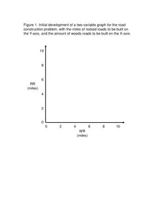
Figure 1. Initial development of a two-variable graph for the road construction problem, with the miles of rocked roads to be built on the Y-axis, and the amount of woods roads to be built on the X-axis. 10. 8. 6. RR (miles). 4. 2. 0. 0. 2. 4. 6. 8. 10. WR (miles).

E N D
Figure 1. Initial development of a two-variable graph for the road construction problem, with the miles of rocked roads to be built on the Y-axis, and the amount of woods roads to be built on the X-axis. 10 8 6 RR (miles) 4 2 0 0 2 4 6 8 10 WR (miles)
Figure 2. The budget constraint for the road construction problem. 10 8 6 RR (miles) 30,000 WR + 50,000 RR 300,000 4 Feasible region 2 0 0 2 4 6 8 10 WR (miles)
Figure 3. A graph of the entire set of constraints to the road construction problem, and the areas related to the constraints where solutions are feasible. 10 8 WR 2.5 WR 6 6 RR (miles) RR 4 4 30,000 WR + 50,000 RR 300,000 2 RR 1.5 0 0 2 4 6 8 10 WR (miles)
Figure 4. Identification of the optimal solution to the road construction problem using a family of objective functions. 10 8 6 RR + WR = 8 RR (miles) 4 RR + WR = 8.4 2 RR + WR = 4 0 0 2 4 6 8 10 WR (miles)
Figure 5. The graphed constraints to the snag development problem, and the identification of the feasible region (gray area). 2,000 CS 250 1,600 1,200 DS (trees) 800 DS 600 100 DS + 50 CS 80,000 400 DS 100 0 0 400 800 1,200 1,600 2,000 CS (trees)
Figure 6. The optimal solution to the snag development problem. 2,000 1,600 1,200 DS (trees) CS + DS = 1,500 800 400 0 0 400 800 1,200 1,600 2,000 CS (trees)
Figure 7. The constraints and feasible region (gray area) associated with the fish habitat problem. Boulders 2.5 25 20 Boulders 7.5 15 Logs (miles) 10,000 Logs + 21,000 Boulders 250,000 10 Logs 5 5 0 0 5 10 15 20 25 Boulders (miles)
Figure 8. Hurricane damage to a pine stand after Hurricane Katrina in 2005.
Figure 9. Identification of the feasible region and optimal solution to the hurricane clean-up problem of cost minimization using a family of objective functions. CH 400,000 1,000,000 CH + CPB 1,000,000 800,000 600,000 CPB 500,000 CPB ($) 400,000 CPB 300,000 200,000 CH + CPB 0 0 200,000 400,000 600,000 800,000 1,000,000 CH ($)
Figure 10. A modified fish habitat problem, with multiple optimal solutions. Boulders 2.5 25 Boulders + Logs 15 20 Boulders 7.5 15 Logs (miles) A 10,000 Logs + 21,000 Boulders 250,000 10 B Logs 5 5 0 0 5 10 15 20 25 Boulders (miles)
Figure 11. An example of efficient, feasible, inefficient, and infeasible solutions to a broad timber harvest and wildlife habitat management problem. B D Timber volume A C (Feasible region solutions) Wildlife habitat
(Figure for question 7) Roads Streams Streams to be treated with logs or boulders