Download
1 / 42
420 likes | 601 Views
Human Chromosomes. Male Xy X y Female XX X XX Xy Daughter Son. Gene, Allele, Genotype, Phenotype. Chromosomes from Father Mother. Genotype Phenotype. Height IQ. AA 185 100 AA 182 104. Gene A , with two alleles A and a.

E N D
Human Chromosomes Male Xy Xy FemaleXXXXXXy Daughter Son
Gene, Allele, Genotype, Phenotype Chromosomes from FatherMother Genotype Phenotype Height IQ AA 185 100 AA 182 104 Gene A, with two alleles A and a Aa 175 103 Aa 171 102 aa 155 101 aa 152 103
Regression model for estimating the genotypic effect Phenotype = Genotype + Error yi = xij + ei xiis the indicator for QTL genotype jis the mean for genotype j ei ~ N(0, 2)
Uniqueness for our genetic problem The genotypes for the trait are not observable and should be predicted from linked neutral molecular markers (M) M1 QTL M2 The genes that lead to the phenotypic variation are called Quantitative Trait Loci (QTL) M3 . . . Our task is to construct a statistical model that connects the QTL genotypes and marker genotypes through observed phenotypes Mm
Parents AA aa F1Aa F2AA Aa aa ¼ ½ ¼ Data Structure n = n22 + n21 + n20 + n12 + n00 + n02 + n01 + n00
Finite mixture model for estimating genotypic effects yi ~ p(yi|,) = ¼ f2(yi) + ½ f1(yi) + ¼ f0(yi) QTL genotype (j) QQQqqq Code 210 where fj(yi) is a normal distribution density with mean jand variance 2 = (2, 1, 0), = (2)
L(, , |M, y) Likelihood function based on the mixture model j|i is the conditional (prior) probability of QTL genotype j (= 2, 1, 0) given marker genotypes for subject i (= 1, …, n).
We model the parameters contained within the mixture model using particular functions QTL genotype frequency: j|i = gj(p) Mean: j= hj(m) Variance: = l(v) • p contains the population genetic parameters • q = (m, v) contains the quantitative genetic parameters
Log- Likelihood Function
The EM algorithm E step Calculate the posterior probability of QTL genotype j for individual i that carries a known marker genotype M step Solve the log-likelihood equations Iterations are made between the E and M steps until convergence
Three statistical issues Modeling mixture proportions, i.e., genotype frequencies at a putative QTL Modeling the mean vector Modeling the (co)variance matrix
Functional Mapping An innovative model for genetic dissection of complex traits by incorporating mathematical aspects of biological principles into a mapping framework Provides a tool for cutting-edge research at the interplay between gene action and development
Parents AA aa F1Aa F2AAAa aa ¼ ½ ¼ Data Structure n = n22 + n21 + n20 + n12 + n00 + n02 + n01 + n00
The Finite Mixture Model Observation vector,yi = [yi(1), …, yi(T)] ~ MVN(uj, ) Mean vector, uj = [uj(1), uj(2), …, uj(T)], (Co)variance matrix,
Modeling the Mean Vector • Parametric approach Growth trajectories – Logistic curve HIV dynamics – Bi-exponential function Biological clock – Van Der Pol equation Drug response – Emax model • Nonparametric approach Lengedre function (orthogonal polynomial) B-spline (Xueli Liu & R. Wu: Genetics, to be submitted)
Stem diameter growth in poplar trees Ma, Casella & Wu: Genetics 2002
Logistic Curve of Growth – A Universal Biological Law (West et al.: Nature 2001) Logistic Curve of Growth – A Universal Biological Law Instead of estimating uj, we estimate curve parameters m= (aj, bj, rj) Modeling the genotype- dependent mean vector, uj = [uj(1), uj(2), …, uj(T)] = [ , , …, ] Number of parameters to be estimated in the mean vector Time points Traditional approach Our approach 5 3 5 = 15 3 3 = 9 10 3 10 = 30 3 3 = 9 50 3 50 = 150 3 3 = 9
Modeling the Variance Matrix Stationary parametric approach Autoregressive (AR) model Nonstationary parameteric approach Structured antedependence (SAD) model Ornstein-Uhlenbeck (OU) process Nonparametric approach Lengendre function
Differences in growth across ages Untransformed Log-transformed Poplar data
Functional mapping incorporated by logistic curves and AR(1) model QTL
Developmental pattern of genetic effects Wu, Ma, Lin, Wang & Casella: Biometrics 2004 Timing at which the QTL is switched on
The implications of functional mapping for high-dimensional biology High-dimensional biology deals with • Multiple genes – Epistatic gene-gene interactions • Multiple environments – Genotype environment interactions • Multiple traits – Trait correlations • Multiple developmental stages • Complex networks among genes, products and phenotypes
Functional mapping for epistasis in poplar Wu, Ma, Lin & Casella Genetics 2004 QTL 1 QTL 2
The growth curves of four different QTL genotypes for two QTL detected on the same linkage group D16
Genotype environment interaction in rice Zhao, Zhu, Gallo-Meagher & Wu: Genetics 2004
Plant height growth trajectories in rice affected by QTL in two contrasting environments Red: Subtropical Hangzhou Blue: Tropical Hainan QQ qq
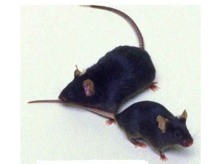
Functional mapping: Genotype sex interaction Zhao, Ma, Cheverud & Wu Physiological Genomics 2004
Body weight growth trajectories affected by QTL in male and female mice QQ Qq qq Red: Male mice Blue: Female mice
Functional mapping for trait correlation Zhao, Hou, Littell & Wu: Biometrics submitted
Growth trajectories for stem height and diameter affected by a pleiotropic QTL Red: Diameter Blue: Height QQ Qq
Statistical Challenges Stem volume = Coefficient Height Diameter2 Logistic curves provide a bad fit of the volume data!
Modeling the mean vector using the Legendre function The general form of a Legendre polynomial of order r is given by the sum, where K = r/2 or (r-1)/2 is an integer. We have first few polynomials: P0(x) = 1 P5(x) = 1/8(63x5-70x3+15x) P1(x) = x P6(x) = 1/16(231x6-315x4+105x2-5) P2(x) = ½(3x2-1) P3(x) = ½(5x3-3x) P4(x) = 1/8(35x4-30x2+3)
New fit by the Legendre function Lin, Hou & Wu: JASA, under revision
Functional Mapping:toward high-dimensional biology • A new conceptual model for genetic mapping of complex traits • A systems approach for studying sophisticated biological problems • A framework for testing biological hypotheses at the interplay among genetics, development, physiology and biomedicine
Functional Mapping:Simplicity from complexity • Estimating fewer biologically meaningful parameters that model the mean vector, • Modeling the structure of the variance matrix by developing powerful statistical methods, leading to few parameters to be estimated, • The reduction of dimension increases the power and precision of parameter estimation
Teosinte and Maize Teosinte branched 1(tb1) is found to affect the differentiation in branch architecture from teosinte to maize (John Doebley 2001)
Biomedical breakthroughs in cancer, next? Single Nucleotide Polymorphisms (SNPs) cancer no cancer Liu, Johnson, Casella & Wu: Genetics 2004 Lin & Wu: Pharmacogenomics Journal 2005