Download
1 / 23
240 likes | 570 Views
Part II: When to Order? Inventory Management Under Uncertainty. Demand or Lead Time or both uncertain Even “good” managers are likely to run out once in a while (a firm must start by choosing a service level/fill rate) When can you run out?

E N D
Part II: When to Order? Inventory Management Under Uncertainty • Demand or Lead Time or both uncertain • Even “good” managers are likely to run out once in a while (a firm must start by choosing a service level/fill rate) • When can you run out? • Only during the Lead Time if you monitor the system. • Solution: build a standard ROP system based on the probability distribution on demand during the lead time (DDLT),which is a r.v. (collecting statistics on lead times is a good starting point!)
The Typical ROP System Average Demand ROP set as demand that accumulates during lead time ROP = ReOrder Point Lead Time
The Self-Correcting Effect- A Benign Demand Rate after ROP Hypothetical Demand Average Demand ROP Lead Time Lead Time
What if Demand is “brisk” after hitting the ROP? Hypothetical Demand Average Demand ROP = EDDLT + SS ROP > EDDLT Safety Stock Lead Time
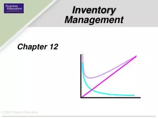
When to Order • The basic EOQ models address how much to order: Q • Now, we address when to order. • Re-Order point (ROP) occurs when the inventory level drops to a predetermined amount, which includes expected demand during lead time (EDDLT) and a safety stock (SS): ROP = EDDLT + SS.
When to Order • SS is additional inventory carried to reduce the risk of a stockout during the lead time interval (think of it as slush fund that we dip into when demand after ROP (DDLT) is more brisk than average) • ROP depends on: • Demand rate (forecast based). • Length of the lead time. • Demand and lead time variability. • Degree of stockout risk acceptable to management (fill rate, order cycle Service Level) DDLT, EDDLT & Std. Dev.
The Order Cycle Service Level,(SL) • The percent of the demand during the lead time (% of DDLT) the firm wishes to satisfy. This is a probability. • This is not the same as the annual service level, since that averages over all time periods and will be a larger number than SL. • SL should not be 100% for most firms. (90%? 95%? 98%?) • SL rises with the Safety Stock to a point.
Safety Stock Quantity Maximum probable demand during lead time (in excess of EDDLT) defines SS Expected demand during lead time (EDDLT) ROP Safety stock (SS) Time LT
Variability in DDLT and SS • Variability in demand during lead time (DDLT) means that stockouts can occur. • Variations in demand rates can result in a temporary surge in demand, which can drain inventory more quickly than expected. • Variations in delivery times can lengthen the time a given supply must cover. • We will emphasize Normal (continuous) distributions to model variable DDLT, but discrete distributions are common as well. • SS buffers against stockout during lead time.
Service Level and Stockout Risk • Target service level (SL) determines how much SS should be held. • Remember, holding stock costs money. • SL = probability that demand will not exceed supply during lead time (i.e. there is no stockout then). • Service level + stockout risk = 100%.
Computing SS from SL for Normal DDLT • Example 10.5 on p. 374 of Gaither & Frazier. • DDLT is normally distributed a mean of 693. and a standard deviation of 139.: • EDDLT = 693. • s.d. (std dev) of DDLT = = 139.. • As computational aid, we need to relate this to Z = standard Normal with mean=0, s.d. = 1 • Z = (DDLT - EDDLT) /
Service level Risk of a stockout Probability of no stockout Quantity ROP Expected demand Safety stock 0 z z-scale Reorder Point (ROP)
Standard Normal(0,1) z-scale 0 z Area under standard Normal pdf from - to +z Z = standard Normal with mean=0, s.d. = 1Z = (X - ) / See G&F Appendix ASee Stevenson, second from last page P(Z <z)
Computing SS from SL for Normal DDLT to provide SL = 95%. • ROP = EDDLT + SS = EDDLT + z (). z is the number of standard deviations SS is set above EDDLT, which is the mean of DDLT. • z is read from Appendix B Table B2. Of Stevenson -OR- Appendix A (p. 768) of Gaither & Frazier: • Locate .95 (area to the left of ROP) inside the table (or as close as you can get), and read off the z value from the margins: z = 1.64. Example: ROP = 693 + 1.64(139) = 921 SS = ROP - EDDLT = 921 - 693. = 1.64(139) = 228 • If we double the s.d. to about 278, SS would double! • Lead time variability reduction can same a lot of inventory and $ (perhaps more than lead time itself!)
Summary View • Holding Cost = C[ Q/2 + SS] • Order trigger by crossing ROP • Order quantity up to (SS + Q) Q+SS = Target Not full due to brisk Demand after trigger ROP = EDDLT + SS ROP > EDDLT Safety Stock Lead Time
Part III: Single-Period Model: Newsvendor • Used to order perishables or other items with limited useful lives. • Fruits and vegetables, Seafood, Cut flowers. • Blood (certain blood products in a blood bank) • Newspapers, magazines, … • Unsold or unused goods are not typically carried over from one period to the next; rather they are salvaged or disposed of. • Model can be used to allocate time-perishable service capacity. • Two costs: shortage (short) and excess (long).
Single-Period Model • Shortage or stockout cost may be a charge for loss of customer goodwill, or the opportunity cost of lost sales (or customer!): Cs = Revenue per unit - Cost per unit. • Excess (Long) cost applies to the items left over at end of the period, which need salvaging Ce = Original cost per unit - Salvage value per unit. (insert smoke, mirrors, and the magic of Leibnitz’s Rule here…)
The Single-Period Model: Newsvendor • How do I know what service level is the best one, based upon my costs? • Answer: Assuming my goal is to maximize profit (at least for the purposes of this analysis!) I should satisfy SL fraction of demand during the next period (DDLT) • If Cs is shortage cost/unit, and Ce is excess cost/unit, then
Single-Period Model for Normally Distributed Demand • Computing the optimal stocking level differs slightly depending on whether demand is continuous (e.g. normal) or discrete. We begin with continuous case. • Suppose demand for apple cider at a downtown street stand varies continuously according to a normal distribution with a mean of 200 liters per week and a standard deviation of 100 liters per week: • Revenue per unit = $ 1 per liter • Cost per unit = $ 0.40 per liter • Salvage value = $ 0.20 per liter.
Single-Period Model for Normally Distributed Demand • Cs = 60 cents per liter • Ce = 20 cents per liter. • SL = Cs/(Cs + Ce) = 60/(60 + 20) = 0.75 • To maximize profit, we should stock enough product to satisfy 75% of the demand (on average!), while we intentionally plan NOT to serve 25% of the demand. • The folks in marketing could get worried! If this is a business where stockouts lose long-term customers, then we must increase Cs to reflect the actual cost of lost customer due to stockout.
Single-Period Model for Continuous Demand • demand is Normal(200 liters per week, variance = 10,000 liters2/wk) … so = 100 liters per week • Continuous example continued: • 75% of the area under the normal curve must be to the left of the stocking level. • Appendix shows a z of 0.67 corresponds to a “left area” of 0.749 • Optimal stocking level = mean + z () = 200 + (0.67)(100) = 267. liters.
Single-Period & Discrete Demand:Lively Lobsters • Lively Lobsters (L.L.) receives a supply of fresh, live lobsters from Maine every day. Lively earns a profit of $7.50 for every lobster sold, but a day-old lobster is worth only $8.50. Each lobster costs L.L. $14.50. • (a) what is the unit cost of a L.L. stockout? Cs = 7.50 = lost profit • (b) unit cost of having a left-over lobster? Ce = 14.50 - 8.50 = cost – salvage value = 6. • (c) What should the L.L. service level be? SL = Cs/(Cs + Ce) = 7.5 / (7.5 + 6) = .56 (larger Cs leads to SL > .50) • Demand follows a discrete (relative frequency) distribution as given on next page.
Lively Lobsters:SL = Cs/(Cs + Ce) =.56 Demand follows a discrete (relative frequency) distribution: Result: order 25 Lobsters, because that is the smallest amount that will serve at least 56% of the demand on a given night.