
GMT 課程
GMT 課程. clipping images using coastlines ( 陸地與海岸的區分 ). PROGS. Palette files. Merging the files themselves may not be doable since they may represent different data sets, Here, we lay down a color map of the geoid field near India with grdimage

GMT 課程
E N D
Presentation Transcript
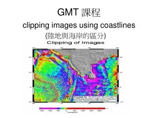
GMT 課程 clipping images using coastlines (陸地與海岸的區分)
PROGS • Palette files. Merging the files themselves may not be doable since they may represent different data sets, • Here, we lay down a color map of the geoid field near India with grdimage • use pscoast to set up land clip paths, and then overlay topography from the TOPO5 data set with another call to grdimage. • We finally undo the clippath with a second call to pscoast with the option –Q
批次檔 • set ingrd1 = india_geoid.grd • set ingrd2 = india_topo.grd • set outgrd1 = india_geoid_i.grd • set outgrd2 = ship_clipped.grd • set outcpt1 = geoid.cpt • set outcpt2 = gray.cpt • set outps1 = example_17.ps • set range1 = 60/90/-10/25 • set proj1 = M6.5i
取得資料來源 • india_geoid.grd → cd/home/GMTDATA/img 切割→grdsample geoid.11.2.grd –G /home/fingerfish/vivico15/ex17/india_ geoid.grd –I6m - R60/90/-10/25 • india_topo.grd 切割→ grdsample TOPO5.GRD -Gindia_topo.grd -I20m -R60/90/-10/25
# First generate geoid image w/ shading • grd2cpt $ingrd1 -Crainbow -V > $outcpt1 • grdgradient $ingrd1 -G$outgrd1 -Nt1 -A45 -V • grdimage $ingrd1 -I$outgrd1 -J$proj1 – C$outcpt1 -P -K -V > $outps1 • psscale -C$outcpt1 -D7/-2/12/0.5h - B500:Topography:/:m: -K -O -V>> $outps1
指令說明 • Read a grdfile and make a color palette file • The cpt file has continuously changing hue (or gray level) and the mapping from data value to hue (or gray level) is through the data's cumulative distribution function (CDF), so that the colors are histogram equalized. • Thus if the resulting cpt file is used with the grdfile and grdimage with a linear projection, the colors will be uniformly distributed in area on the plot.
# Then use pscoast to initiate clip path for land • pscoast -R$range1 -JM -Dl -Gc -O -K -V >> $outps1 • -Gc→clipping of "dry" areas • if -Sc→ clipping of ""wet" areas • ingrd1 ↔ ingrd2 • outgrd1 ↔ outgrd2 • outcpt1 ↔ outcpt1
# Now generate topography image w/shading • echo "-10000 150 10000 150" > $outcpt2 • grdgradient $ingrd2 -G$outgrd2 -Nt1 -A45 -V • grdimage $ingrd2 -I$outgrd2 -JM -C$outcpt2 -O -K -V >> $outps1
# Finally undo clipping and overlay basemap • pscoast -R -JM -Q -B10f5:."Clipping of Images": -O -K -V >> $outps1 • -Q →Mark end of existing clip path. Noprojection information is needed.
# Add a text paragraph 方框的高度 方框的寬度 • pstext -R -JM -O -M -W255O0.5p -D-0.1i/0.1i -V << EOF >> $outps1 • > 90 -10 12 0 4 RB 12p 3i j • @_@%5%Example 17.@%%@_ We first plot the color geoid image for the entire region, followed by a gray-shaded @#etopo5@# image that is clipped so it is only visible inside the coastlines. EOF
#\rm -f geoid.cpt gray.cpt *_i.grd • #imagetool $outps1 & gv $outps1 &
報告完畢~~ 謝謝!