Lecture 15: Eigenfaces
390 likes | 793 Views
CS6670: Computer Vision. Noah Snavely. Lecture 15: Eigenfaces. Announcements. Final project page up, at http://www.cs.cornell.edu/courses/cs6670/2009fa/projects/p4/ One person from each team should submit a proposal (to CMS) by tomorrow at 11:59pm Project 3: Eigenfaces.

Lecture 15: Eigenfaces
E N D
Presentation Transcript
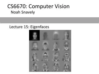
CS6670: Computer Vision Noah Snavely Lecture 15: Eigenfaces
Announcements • Final project page up, at • http://www.cs.cornell.edu/courses/cs6670/2009fa/projects/p4/ • One person from each team should submit a proposal (to CMS) by tomorrow at 11:59pm • Project 3: Eigenfaces
H. Schneiderman and T.Kanade General classification • This same procedure applies in more general circumstances • More than two classes • More than one dimension • Example: face detection • Here, X is an image region • dimension = # pixels • each face can be thoughtof as a point in a highdimensional space H. Schneiderman, T. Kanade. "A Statistical Method for 3D Object Detection Applied to Faces and Cars". IEEE Conference on Computer Vision and Pattern Recognition (CVPR 2000) http://www-2.cs.cmu.edu/afs/cs.cmu.edu/user/hws/www/CVPR00.pdf
convert x into v1, v2 coordinates What does the v2 coordinate measure? • distance to line • use it for classification—near 0 for orange pts What does the v1 coordinate measure? • position along line • use it to specify which orange point it is Linear subspaces • Classification can be expensive • Must either search (e.g., nearest neighbors) or store large PDF’s • Suppose the data points are arranged as above • Idea—fit a line, classifier measures distance to line
Dimensionality reduction How to find v1 and v2 ? • Dimensionality reduction • We can represent the orange points with only their v1 coordinates • since v2 coordinates are all essentially 0 • This makes it much cheaper to store and compare points • A bigger deal for higher dimensional problems
Linear subspaces Consider the variation along direction v among all of the orange points: What unit vector v minimizes var? What unit vector v maximizes var? 2 Solution: v1 is eigenvector of A with largest eigenvalue v2 is eigenvector of A with smallest eigenvalue
Principal component analysis • Suppose each data point is N-dimensional • Same procedure applies: • The eigenvectors of A define a new coordinate system • eigenvector with largest eigenvalue captures the most variation among training vectors x • eigenvector with smallest eigenvalue has least variation • We can compress the data by only using the top few eigenvectors • corresponds to choosing a “linear subspace” • represent points on a line, plane, or “hyper-plane” • these eigenvectors are known as the principal components
= + The space of faces • An image is a point in a high dimensional space • An N x M intensity image is a point in RNM • We can define vectors in this space as we did in the 2D case
Dimensionality reduction • The set of faces is a “subspace” of the set of images • Suppose it is K dimensional • We can find the best subspace using PCA • This is like fitting a “hyper-plane” to the set of faces • spanned by vectors v1, v2, ..., vK • any face
Eigenfaces • PCA extracts the eigenvectors of A • Gives a set of vectors v1, v2, v3, ... • Each one of these vectors is a direction in face space • what do these look like?
Projecting onto the eigenfaces • The eigenfaces v1, ..., vK span the space of faces • A face is converted to eigenface coordinates by
Detection and recognition with eigenfaces • Algorithm • Process the image database (set of images with labels) • Run PCA—compute eigenfaces • Calculate the K coefficients for each image • Given a new image (to be recognized) x, calculate K coefficients • Detect if x is a face • If it is a face, who is it? • Find closest labeled face in database • nearest-neighbor in K-dimensional space
i = K NM Choosing the dimension K • How many eigenfaces to use? • Look at the decay of the eigenvalues • the eigenvalue tells you the amount of variance “in the direction” of that eigenface • ignore eigenfaces with low variance eigenvalues
Issues: metrics • What’s the best way to compare images? • need to define appropriate features • depends on goal of recognition task classification/detectionsimple features work well(Viola/Jones, etc.) exact matchingcomplex features work well(SIFT, MOPS, etc.)
Metrics • Lots more feature types that we haven’t mentioned • moments, statistics • metrics: Earth mover’s distance, ... • edges, curves • metrics: Hausdorff, shape context, ... • 3D: surfaces, spin images • metrics: chamfer (ICP) • ...
If you have a training set of images:AdaBoost, etc. Issues: feature selection If all you have is one image:non-maximum suppression, etc.
Issues: data modeling • Generative methods • model the “shape” of each class • histograms, PCA, mixtures of Gaussians • graphical models (HMM’s, belief networks, etc.) • ... • Discriminative methods • model boundaries between classes • perceptrons, neural networks • support vector machines (SVM’s)
Generative vs. Discriminative Generative Approachmodel individual classes, priors Discriminative Approachmodel posterior directly from Chris Bishop
Issues: dimensionality • What if your space isn’t flat? • PCA may not help Nonlinear methodsLLE, MDS, etc.
Issues: speed • Case study: Viola Jones face detector • Exploits two key strategies: • simple, super-efficient features • pruning (cascaded classifiers) • Next few slides adapted Grauman & Liebe’s tutorial • http://www.vision.ee.ethz.ch/~bleibe/teaching/tutorial-aaai08/ • Also see Paul Viola’s talk (video) • http://www.cs.washington.edu/education/courses/577/04sp/contents.html#DM
Feature extraction “Rectangular” filters • Feature output is difference between adjacent regions Value at (x,y) is sum of pixels above and to the left of (x,y) • Efficiently computable with integral image: any sum can be computed in constant time • Avoid scaling images scale features directly for same cost Integral image Viola & Jones, CVPR 2001 22 K. Grauman, B. Leibe K. Grauman, B. Leibe
Large library of filters • Considering all possible filter parameters: position, scale, and type: • 180,000+ possible features associated with each 24 x 24 window Use AdaBoost both to select the informative features and to form the classifier Viola & Jones, CVPR 2001 K. Grauman, B. Leibe
AdaBoost for feature+classifier selection Want to select the single rectangle feature and threshold that best separates positive (faces) and negative (non-faces) training examples, in terms of weighted error. Resulting weak classifier: For next round, reweight the examples according to errors, choose another filter/threshold combo. … Outputs of a possible rectangle feature on faces and non-faces. Viola & Jones, CVPR 2001 K. Grauman, B. Leibe
AdaBoost: Intuition Consider a 2-d feature space with positive and negative examples. Each weak classifier splits the training examples with at least 50% accuracy. Examples misclassified by a previous weak learner are given more emphasis at future rounds. Figure adapted from Freund and Schapire 25 K. Grauman, B. Leibe K. Grauman, B. Leibe
AdaBoost: Intuition 26 K. Grauman, B. Leibe K. Grauman, B. Leibe
AdaBoost: Intuition Final classifier is combination of the weak classifiers 27 K. Grauman, B. Leibe K. Grauman, B. Leibe
AdaBoost Algorithm Start with uniform weights on training examples {x1,…xn} For T rounds Evaluate weighted error for each feature, pick best. Re-weight the examples: Incorrectly classified -> more weight Correctly classified -> less weight Final classifier is combination of the weak ones, weighted according to error they had. Freund & Schapire 1995 K. Grauman, B. Leibe
Cascading classifiers for detection Fleuret & Geman, IJCV 2001 Rowley et al., PAMI 1998 Viola & Jones, CVPR 2001 For efficiency, apply less accurate but faster classifiers first to immediately discard windows that clearly appear to be negative; e.g., • Filter for promising regions with an initial inexpensive classifier • Build a chain of classifiers, choosing cheap ones with low false negative rates early in the chain 29 Figure from Viola & Jones CVPR 2001 K. Grauman, B. Leibe K. Grauman, B. Leibe
Viola-Jones Face Detector: Summary Train cascade of classifiers with AdaBoost Apply to each subwindow Faces New image Selected features, thresholds, and weights Non-faces Train with 5K positives, 350M negatives Real-time detector using 38 layer cascade 6061 features in final layer [Implementation available in OpenCV: http://www.intel.com/technology/computing/opencv/] 30 K. Grauman, B. Leibe
Viola-Jones Face Detector: Results First two features selected 31 K. Grauman, B. Leibe K. Grauman, B. Leibe
Viola-Jones Face Detector: Results K. Grauman, B. Leibe
Viola-Jones Face Detector: Results K. Grauman, B. Leibe
Viola-Jones Face Detector: Results K. Grauman, B. Leibe
Detecting profile faces? Detecting profile faces requires training separate detector with profile examples. K. Grauman, B. Leibe
Viola-Jones Face Detector: Results Paul Viola, ICCV tutorial K. Grauman, B. Leibe