Download
1 / 76
810 likes | 1.08k Views
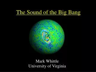
The Sound of the Big Bang. Mark Whittle University of Virginia. The roots of cosmic structure. How did the Universe go from so smooth to so lumpy ??. Complex topic, with many parts. Our approach is gradual, Whenever possible: illustrate with sounds :

E N D
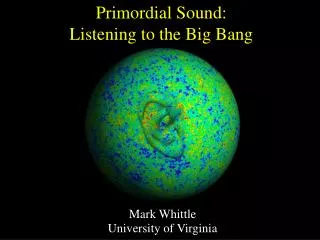
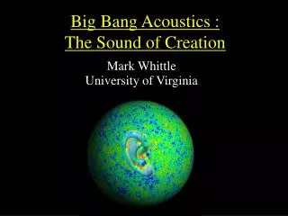
The Sound of the Big Bang Mark Whittle University of Virginia
The roots of cosmic structure How did the Universe go from so smooth to so lumpy ?? • Complex topic, with many parts. Our approach is gradual, • Whenever possible: illustrate with sounds : • The Cosmic Microwave Background (CMB) • Anisotropies as seeds & sound • Growth of fluctuations : super- & sub- horizon. • Cosmic diagnostics: the concordance model • Bumps & wiggles in C(ℓ) • Removing distortions: C(ℓ) P(k) • Evolving P(k): the first 400 kyr • Fun with chords – musical analysis. • From sound to stars : the first 100 Myr • The initial power spectrum: inflation & quantum hiss
Disclaimer: I am not a CMB specialist! • this began in 2003 as public outreach, following WMAP. • However, there are two publics: • the “true” public • the “other” public: non-CMB astronomers/physicists • (who, like me, easily get confused by all the details) • This is aimed at the latter group: • an overview of the CMB, with sound & movies for fun. Acknowledgments: Joe Wolfe & Alex Tarnopolsky (UNSW) for help with acoustics. Constantinos Skordis (Oxford) for help with CMBFAST & DASh. Charlie Lineweaver (UNSW), Pedro Ferreira (Oxford) & Louise Ord (UNSW), for help with CMB physics. Howard Powell and Mike Tuite (UVa) for help with images and movie making.
red-shift Our view of the Universe includes space and time The Early Universe was filled with hot glowing gas
expansion cooling Big Bang dense hot rarified cool Now ionized foggy 380,000 yr 3000 K hot glowing fog us redshift z=1000 Making the CMB atomic transparent we see a glowing wall of bright fog orange light microwaves
Human lifespan Conc- eption child teenage Old age 12hr Marathon race Finish 26 miles Start 4 feet CMB is Young and Far 380,000 yr 5 Time (Gyr) 10 0 14 Big Bang here now “nearby” galaxies CMB NGST HST
Bell Labs (1963) Observing the Microwave Background (highlights, there are many others) COBE satellite (1992) WMAP satellite (2003)
The Celestial Sphere Optical Sky Microwave Sky Microwave Sky Stretched
Two ways to view patchiness • Seeds of cosmic structure : • Gravity amplifies density variations • peaks galaxies; troughs voids • 2. Sound waves : • peaks & troughs in pressure = sound waves • the “Big Bang” has both light and sound • acoustic analysis reveals cosmic properties
Sound waves in the sky Water waves : high/low level of water surface Many waves of different sizes, directions & phases all “superposed” Sound waves : red/blue = high/low gas & light pressure
A I N B B G G S A C C O I U T I T What, me worry? S
What does the CMB “sound” like? Three important aspects to perceived sound: Volume Pitch Quality (color) Consider each in turn:
How Loud is the Sound? • Consider decibel scale: • Human ear, threshold of hearing: Ilim ~ 10-12W m-2 • corresponds toΔP/Po ~ 2× 10⁻¹⁰ • LdB = 10 log10 (I / Ilim) = 20 log10(ΔP/ΔPlim) • range 0140 dB : ΔP/Po ~ 10-10 10-3 (10-12102 Wm-2) • human ears are sensitive with high dynamic range @ CMB : Po ~ 10-7atm (Prad/Pgas ~ nγ/np ~ 109) Fluctuations:ΔT/To ~ 1–5 × 10⁻⁵&ΔP/Po = 4ΔT/To ΔP/Po ~ 4–20 × 10-5 ≡ 100–120 dB Quite loud !!
What Pitch is the Sound? CMB observed frequencies : all sky –sub-horizon θ : angle on sky (~180°/ℓ) 90° – 2° – 0.1° ℓ : harmonic frequency 2 – 50 – 2000 λ : wavelength (h-1 Mpc) 5 Mpc – 380 kly – 20 kly λco: comoving length 5000 – 120 – 3 Mpc kco: wave # (2π/λco, log10) -3.7 – -2.1 – -0.7 f : frequency (Hz) ~ vs/λ *10-14.5 – 10-13 – 10-11.5 P : Period (1/f, kyr) 10 Myr –300 – 10 kyr octaves below A (440Hz) 57 –52 – 47 range (dex / octaves) 3 / 101.5 / 5 * Sound speed : vs ~ c / (3 + 9ρb/4ργ)½ = (1 → 0.84) × c /√3
Transposing in Pitch The CMB sounds are way too deep to hear !! Human ear range: ~ 10 Hz – 10 kHz ie ~ 3 dex ~ 10 octaves (210 = 1024) cf piano : ~ 7 octaves, ~ 27 Hz – 4 kHz (~A440 ± 4 oct) Range of CMB data is well matched to human ear ! Choose to map ℓ→ Hz : transpose up by ~50 octaves super-horizon : ℓ~ 2 – 50 ≡ 2 – 50 Hz ~ sub-audible 1st acoustic peak : ℓ~ 220 ≡ 220 Hz = A below A440 highest notes : ℓ~ 2000 ≡ 2 kHz ~2.2 oct above A440 leaves space (2 – 10 kHz) for earlier epochs
DEEP? Why is primordial sound so BIG Because the Universe is so: Cathedral Organ Universe Pan Pipes Recorders 400,000 light years
7 octaves 7 octaves 7 octaves 7 octaves 7 octaves 7 octaves 7 octaves Transpose up by ~50 octaves = 7 pianos (~7 octaves each) cosmic concerto human concerto deeper An Ultra-BassPiano
Sound quality: power spectra There are many frequencies present. The relative amount of each sound quality This is called the power spectrum : P(λ)≡P(k) Waveform Fourier Transform Power Spec. (pressure vs time) (loudness vs freq.) Two examples :
Flute & Clarinet sound spectra Joe Wolfe (UNSW) Bь Clarinet piano range Modern Flute
Sky Maps Power Spectra Cannot follow waves in time. Instead use the wave’s spatial appearance Evaluate spatial power spectrum, of waves on the sphere. “frequency” is spherical angular harmonic: ℓ peak trough Lineweaver 1997
More formally: “Fourier” approach to functions on a sphere: For CMB, usually plot: ℓ(ℓ+1) C(ℓ) vs ℓ [μK2] [ Because P(k) ~ kn (n~1) projects to C(ℓ) ~ const / ℓ(ℓ+1) ]
The Observed Sound Spectrum current best data × ( model) angular wavelength (degrees) fundamental harmonics Sound “Loudness” sky frequency (~180/°)
From PS to sound: • Relatively straightforward: • Choose time step ~0.05 ms (20 kHz sample rate) • For each time step: • add 2000 sine functions (one for each ℓ) • each has frequency & amplitude defined by P.S. • each has random phase Finally: S(ti) ascii array “sox” utility sound.wav
current best data × “concordance” model A 220 Frequency (in Hz) CMB Angular Sound Spectrum Lineweaver 2003 Frequency (on the sky)
Sound Waves in the Sky The CMB Power Spectrum Relative loudness at different pitch NASA’s WMAP satellite sound Loudspeaker Loudness Raw CMB sound Frequency Wavelength Lower Pitch Higher Pitch The Microwave Sky Water waves on the ocean surface illustrate sound waves on the CMB “surface” short plus medium plus long all mixed together Microwave brightness, greatly contrast stretched. Brightness differences are also pressure differences Patches smaller than 2º are sound waves
Growth of initial fluctuations • Early Universe was extremely smooth • However, not perfectly smooth (fortunately for us) • “Initial” irregularities come from inflation (see later) • Very small Δρ/ρ variations exist on all scales: • P(k) ~ kn≡ P(λ) ~ λ-n(n~1 = Harrison-Zeldovich spectrum) • All components vary in step: cdm / baryons / γs / νs • curvature fluctuations (also called “adiabatic”) expansion lags/leads from location to location • fluctuations grow on all scales: Δρ/ρ ~ R2 • Fluctuations haverandom phase • patchiness is random (no-one’s name is spelled out) • on all scales, amplitude distribution is Gaussian
The Horizon • The horizon size separates two very different scales: • Small scales gravitationally connected (sub-horizon) • Large scales gravitationally unconnected (super-horizon) • The horizon size grows at light speed: rH ~ ctage • When a wavelength “enters the horizon” it can respond to itself and other nearby perturbations • eg gas can fall into potential wells (valleys) entering horizon ctage outside horizon inside horizon
compression dim dim rarefaction bright rarefaction bright bright rarefaction compression compression dim The first sound waves • gas falls into valleys, gets compressed, & glows brighter b) it overshoots, then rebounds out, is rarefied, & gets dimmer c) it then falls back in again to make a second compression the oscillation continues sound waves are created • Gravity drives the growth of sound in the early Universe. • The gas must also exert pressure, so it rebounds out of the valleys. • We see the bright/dim regions as patchiness on the CMB.
C(ℓ) as cosmic diagnostic • For any object, P.S. depends on structure • e.g. flute & clarinet playing G# have different P.S. • understanding the P.S. structure of object • Likewise, CMB P.S. structure of universe • Combine several datasets (including CMB) • ~12 parameters with high accuracy. • Concordance model • Two examples with clear acoustic signature :
7 Total Cosmic Density reality Low pitch Long Wavelength High pitch Short Wavelength
Geometry & Sound Pitch Region size ~ outstretched hand Real Data Simulated data for different densities “critical” flat geometry flat lens medium blobs medium pitch high density +ve curvature convex lens big blobs deep pitch low density -ve curvature concave lens small blobs high pitch
7 Fraction of Baryons (detail) reality Low pitch Long Wavelength High pitch Short Wavelength
Properties from the CMB • Age of Universe13.7 Gyr (2%) • Flatness 1.02 (2%) • Atoms 4.4% (9%) • Dark matter 23% (15%) • Dark energy 73% (5%) • Hubble constant (km/s/Mpc) 71 (6%) • Photon/proton ratio 1.6x10⁹ (5%) • Time of first stars 180 Myr (50%) • Time of MWB 380,000yr (2%)
5. Understanding C(ℓ) What are all those bumps & wiggles??
(1) (2) Φ cold hot Sachs Wolfe Understanding C(ℓ) • What are all those bumps and wiggles ?? • Many processes affect C(ℓ), not all are sound waves !! • Usually divided: Primary/Secondary/(Tertiary) • Primary: • more/less dense (valley/hill) hot/cold blue/red • valley/hill gravitational red/blue shift • these partly cancel: • (sub & super horizon) • gas falls in / rebounds out Doppler red/blue shift • (sub-horizon only, ie ℓ > 50) • formation of fundamental & harmonics
Origin of Fundamental & Harmonics Large scales Radiation dominated Recombination Matter dominated Doppler blurring Lineweaver 1997 first compression peak = fundamental Doppler blurring first rarefaction peak smaller region rarefaction rebound compression infall start Small scales Visible Wall Collapse Begins Foggy & Hidden
Understanding C(ℓ) • Secondary: • Smearing : λ < ΔRrec wash out; kills high ℓ • Silk damping: photon diffusion, kills high ℓ • Integrated Sachs-Wolfe: γs cross varying Φ • Early ISW : Φγ near zrec (adds power @ ℓ~100) • Late ISW : Λ → Φ(z<1) (adds power @ ℓ<10) • Rees-Sciama : Φ from proto-clusters (small effect) • Re-ionization : @ z~20 lowers power for λ < λH(zre-ion) • ClusterSZeffects : add power @ high ℓ >3000 · · • Tertiary(contamination): • Galactic: dust, free-free, synchrotron • Point sources: radio galaxies; high-z IR gals • Dipole (10-3× Tcmb ; 102× other anisotropies)
Acoustic & Doppler sub- super- horizon Δzrec smearing Silk damping Late ISW Early ISW SW plateau
The cosmic concert hall • The observed P.S. isn’t purely acoustic • The universe is not a perfect concert hall : eg audience cough and fidget [foreground galaxy] carpet/drapes deaden sound [Silk damping] Correct both : use spectral differences to remove galaxy use computer simulations to remove distortions Observed : C(ℓ) Pure : P(k)
Modeling C(ℓ) and P(k) • Highly sophisticated; long history: Early work: Peebles; Silk; Bond; Efstathiou….. Developments: Seljak; Sugiyama; Zaldarriaga; Hu…….. Improved numerical methods & physical understanding • Public code : CMBFAST (Seljak & Zaldarriaga ‘96) • In theory: • 4 fluids: CDM & υs (collisionless); baryons & γs (collisional) Evolve fluid DFs using Boltzmann Eqn + perturbations P(k,z) & Transfer functions → C(ℓ) • Physics “known” → accurate to ≤ few % • In practice: • Input global: Ωb Ωm ΩΛ Ων Tcmb h; & perturbations: n, A, type. • Let rip P(k,z) for baryons, γ, cdm, υ; + C(ℓ)
fundamental Flute Universe C(ℓ) h a r m o n i c s P(k) Why does it sound so “unmusical”? • Because the Universe is not a good resonator • the harmonics are broad (fuzzy) • we do not easily notice the hidden notes Compare the Universe with a flute: decibel scales
A “broad” note sounds quite different from a pure tone The difference seems greatest for the lowest note. Single tone Pure sine wave Spread of tones ~200 Hz range
What’s the Chord ? } Between major & minor 3rd C(ℓ) as observed P(k) undistorted P(k) pure tones