Download

1 / 71
760 likes | 1.02k Views
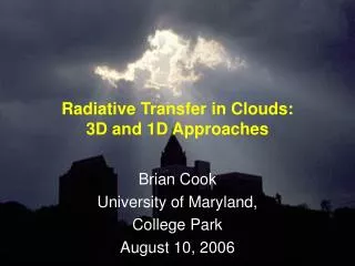
Three-Dimensional Radiative Transfer in Clouds. Warren Wiscombe NASA Goddard. dedicated to Gerry Pomraning and Georgii Titov. See new book, edited by Marshak and Davis, published late 2004. mainly shortwave (sunlight).

E N D
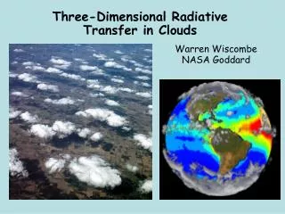
Three-Dimensional Radiative Transfer in Clouds Warren Wiscombe NASA Goddard
dedicated to Gerry Pomraning and Georgii Titov See new book, edited by Marshak and Davis, published late 2004 • mainly shortwave (sunlight) 3D Rad Transf in Clouds
A motivation: Clouds cause 2–5 C range in predicted global average temperature increase for 2xCO2 1979 Report on CO2 and Climate, Woods Hole: “... the equilibrium surface global warming due to 2xCO2 will be in the range 1.5 to 4.5 C”. 2001 IPCC: Essentially the same as above. temperature range is pretty uniformly filled! 3D Rad Transf in Clouds
99% of atmospheric radiative transfer approximate{d,s} 3D clouds as 1D slabs Constraints were: slow computers, and inability to (a) specify cloud in 3D, (b) test models (cloud or radiation) 3D Rad Transf in Clouds
There’s an approximately 1D world overhead on a mountaintop on a clear day 3D Rad Transf in Clouds
But the real world of cloud radiation looks nothing like the tame, peaceful 1D world 3D Rad Transf in Clouds
What are the unique aspects of Earth atmospheric radiative transfer? • Clouds & vegetation — extreme 3D, big scale range • Strong, dense absorption lines • Forward-peaked scattering phase function • Surface BRDF important • specular reflection, hot spot! • Polarization — Rayleigh, aerosol, glint • Beams from inside, outside • Rapid variation — turbulent 3D Rad Transf in Clouds
Real cloud radiation looks turbulent, with occasional excursions above the 1D envelope 3D Rad Transf in Clouds
and it still looks intermittent for a 3–hr subset of total flux! 3D Rad Transf in Clouds
1D radiative transfer history in the atmospheric sciences • Chandrasekhar (1950): • polarized radiative transfer • Sekera & students (1950s) inspired by Chandrasekhar to study Rayleigh scattering atmosphere w. aerosol • polarized r.t. survived only in microwave until POLDER reinvigorated field • van de Hulst, Twomey (1960s): adding-doubling • Dave and others: spherical harmonics w. polarization • 1968 code still survives in UV project at Goddard! • Dave: Mie scattering 3D Rad Transf in Clouds
Peaks of 1D theory were reached with • Grant-Hunt version of adding-doubling (1969) • Stamnes et al. discrete ordinates (DISORT, 1988) • k-distributions (Lacis/Hansen and others, 1980s) Atmospheric radiative transfer field focused on the wavelength rather than the x-y spatial dimension. Lab spectroscopy measurements led to an hubris that models were correct without testing them in the open air. Thus the field became largely an indoor activity... 3D Rad Transf in Clouds
Thus, when theoreticians emerged into the open air, they were puzzled... “What is this strange alien object?” 3D Rad Transf in Clouds
I started in 3D and 1D-spherical r.t., devolved to 1D-slab... • In 1970, the 3D world I entered was dominated by • Monte Carlo methods • discretize everything • spectral-expand some things, discretize others • diffusion, Eddington methods & variants • First two were severely computer-constrained • random number generators were mediocre • linear algebra algorithms for large matrices were poor (this was even before LINPACK!) • Atmospheric science inherited these methods but eventually improved on them considerably 3D Rad Transf in Clouds
then I rode the 1D to 3D transition in cloud radiation, mainly funded by ARM • In radiative transfer methodology, the transition was somewhat predictable: • more photons in Monte Carlo (finally, enough!) • various stews of discrete vs. spectral for both angle and space dimensions, with some computationally hopeless, now-dead methods • avoidance of brute force methods because matrices can become so large (a small problem of 100x100x20 w. 80 discrete angles could lead to matrices of 16Mx16M) 3D Rad Transf in Clouds
The full range of 3D radiative transfer options are now used in cloud studies • Diffusion and other approximations • Analytical-numerical (quintessence: SHDOM, 1998) • Monte Carlo + Open source Monte Carlo • Cases: • step cloud • 2D field from ARM radar • 3D field derived from Landsat • Sc and shallow Cu, Large Eddy model 3D Rad Transf in Clouds
Emerging subject, cloud micro-3D radiative transfer, challenges “elementary-volume” assumption embodied in phase function p • Monochromatic Radiative Transfer Equation 3D Rad Transf in Clouds
What assumptions are being challenged? • NumberOfDrops(radius r) = cxVolume • According to high-time-resolution aircraft data, above a critical radius of ~14 mm: • NumberOfDrops(radius r) = c(r) xVolumeD(r) where 0 < D(r) < 1 • (2) the larger drops are, the more they cluster 3D Rad Transf in Clouds
This is a numerical simulation of drop clustering based on aircraft data 3D Rad Transf in Clouds
But if we give up “elementary volume”, what can we do, radiative transfer-wise? • First-principles Monte Carlo: each photon interacts with actual drops at specific spatial locations, rather than with a fictitious elementary volume. • (At the outermost limit of what we can do computationally) • Fractional differential equations: in the very simplest case of pure transmission through a fractal-clustered drop distribution, must solve: 3D Rad Transf in Clouds
Many details of 3D radiative transfer will be covered in the following talks, so because the 1D to 3D transition in cloud structure modeling was more unexpected, I will focus instead on: cloud structure — theoreti-empirical, and instruments for measuring it tentative steps toward incorporating 3D into routine activities of our field 3D Rad Transf in Clouds
Clouds are highly variable in x, y, z & t • “Immense chaos amid immense order” (turbulence produces chaos, reigned in by overall physical controls that create & sustain large cloud systems) • Clouds are the tip of the water vapor iceberg! • Typically <3% of water vapor in column condenses. • Clouds represent only the tail of the relative humidity probability distribution; this already ensures high variability. 3D Rad Transf in Clouds
Real regularity in clouds happens when waves overpower turbulence, and is rare 3D Rad Transf in Clouds
This deep tropical convection from Shuttle is more typical of the “immense chaos” 3D Rad Transf in Clouds
Coast of Holland shows how surface variability adds to cloud variability • These cloud waves would cause mild bump in power spectrum Landsat image 3D Rad Transf in Clouds
Nevertheless, following Occam’s Razor, clouds were modeled as cubes, 1975-90 3D Rad Transf in Clouds
the ultimate Euclidean cloud... 3D Rad Transf in Clouds
Lovejoy (1982) showed that clouds have a fractal not Euclidean character • if Euclidean: • area µ perim2 • the data show: • area µ perim1.5 3D Rad Transf in Clouds
What other evidence of fractality was found? Cloud liquid water power spectra from field campaigns: - scaling behavior over a range 10 m to ~50 km! - no preferred scale 3D Rad Transf in Clouds
How was the idea of modeling clouds as fractals received? • Euclidean cloud papers survived into the early 1990s • Fractal models not taken seriously until extended: • beyond the monofractals in Mandelbrot’s book • beyond cloud geometry, to cloud liquid water • Two attractive features finally won the day: • simpler than Euclidean models (fewer parameters) • better connected to the underlying scaling physics exemplified in Kolmogorov approach to turbulence 3D Rad Transf in Clouds
Nowadays we routinely model statistical clouds using empirical information 3D Rad Transf in Clouds
Scaling analysis for Landsat cloud radiances revealed a scale break at ~0.5 km...not seen in cloud optical depth. 3D Rad Transf in Clouds
3D radiative smoothing has three regimes Analysis of the Landsat scale break led to the basic ideas underlying multiple scattering lidar 3D Rad Transf in Clouds
Another way to specify a cloud is to use a “cloud-resolving model” Dynamical and dynamical/microphysical cloud models were mainly for thunderstorms. Models for more horizontally extensive cloud forms remained primitive through the 1980s, but have matured since then and are now routinely used to provide input to 3D radiative transfer models. Most 3D radiation modelers use both fractal and cloud-resolving models for specifying clouds, according to the situation. 3D Rad Transf in Clouds
Ron Welch, Bill Hall and I pioneered radiation-cloud physics collaboration • Hall/Clark model: • 2D thunderstorm! • explicit drop size categories • We horizontally averaged Hall’s results to use in a 1D radiation model — ugh... 3D Rad Transf in Clouds
I3RC (Intercomparison of 3D Radiation Codes) uses cloud-resolving model input for some cases http://i3rc.gsfc.nasa.gov/ 3D Rad Transf in Clouds
What simple ways have been put forward to deal with or account for 3D variability in climate models? 3D Rad Transf in Clouds
1D error has two very different natures depending on pixel size Independent Column Plane-Parallel 3D Rad Transf in Clouds
Cubic clouds gave an extreme view of the perils of ignoring 3D cloudy cubes have optical depth 50 3D Rad Transf in Clouds
The simplest and oldest method for dealing with 3D is “cloud fraction” Cloud fraction (“oktas”) has sentimental and historical value in meteorology. Cloud fraction Ac is used as a linear weight: 3D Rad Transf in Clouds
So what’s wrong with cloud fraction? Stephens (1988), showed that (equality only when no correlations between fluctuations in the radiation and cloud fields) This inequality makes it impossible to test retrievals of Ac(radiative) against an alternative, non-radiative definition. (done still) Sometimes Ac(radiative) < 0 to get the radiation right! 3D Rad Transf in Clouds
The next band-aid beyond cloud fraction was cloud overlap random, maximum, and max-random were all tried...but none seem to work well 3D Rad Transf in Clouds
The first decent 1D approximation to 3D was the Independent Column Approximation (ICA) Requires the probability distribution of optical depth pdf(t) in the cloudy part of the scene, instead of just the mean optical depth. Since the low-t part of pdf(t) is very hard to get, in practice we still fall back on cloud fraction... 3D Rad Transf in Clouds
100-500 km Application to Global Climate Models • Approximations to incorporate 3D effects into a 1D framework: • Cahalan, • Barker/Oreopoulis, • Cairns, • Pincus/Barker. 3D Rad Transf in Clouds
Serious limitation of slab model is partitioning of space into two disjoint half-spaces, one containing Sun, other the Earth so from any point, can view reflected or transmitted light, not both Davis has proposed a spherical cloud model more in accord with everyday experience 3D Rad Transf in Clouds
Davis uses illuminated and shaded sides of each cloud to retrieve “optical diameter” generalization of familiar 2-stream theory with redefintion of R, T, t 3D Rad Transf in Clouds
How do 3D effects impact typical 1D retrievals of cloud properties? 3D Rad Transf in Clouds
1D retrieval of cloud optical depth at increasingly oblique angles shows 3D effect 3D Rad Transf in Clouds
Remote retrieval of cloud optical depth t using 1D algorithms incurs considerable bias • Each dot corresponds to a 50x50 km area with t averaged separately over all illuminated vs all shaded pixels 3D Rad Transf in Clouds
Cahalan inhomogeneity parameter c is rough measure of 3D bias in optical depth where t is cloud optical depth 3D Rad Transf in Clouds
What instruments do we currently use to probe and characterize clouds? • Major categories are passive & active (probes) • We must extrapolate 1D or 2D data into 4D: • ground-based probes: t-z • aircraft-based probes: mix of t–z and x–z • space-based probes: x-z • all are dimensionally challenged! 3D Rad Transf in Clouds