Download

1 / 68
690 likes | 872 Views
High Bandwidth Instruction Fetching Techniques. Instruction Bandwidth Issues The Basic Block Fetch Limitation Requirements For High-Bandwidth Instruction Fetch Units Multiple Branch Prediction Interleaved Sequential Core Fetch Unit Enhanced Instruction Caches: Collapsing Buffer (CB)

E N D
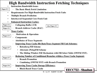
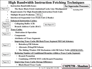
High Bandwidth Instruction Fetching Techniques • Instruction Bandwidth Issues • The Basic Block Fetch Limitation • Requirements For High-Bandwidth Instruction Fetch Units • Multiple Branch Prediction • Interleaved Sequential Core Fetch Unit • Enhanced Instruction Caches: • Collapsing Buffer (CB) • Branch Address Cache (BAC) • Trace Cache: • Motivation & Operation • Components • Attributes of Trace Segments • Improving Trace Cache Hit Rate/Trace Segment Fill Unit Schemes: • Rotenberg Fill Scheme • Alternate (Pelog)Fill Scheme • The Sliding Window Fill Mechanism with Fill Select Table (SWFM/ FST). • Reducing Number of Conditional Branches within a Trace Cache Segment: • Branch Promotion • Combining (SWFM/ FST) with Branch Promotion • Improving Trace Cache Storage Efficiency: • Block-Based Trace Cache
Decoupled Fetch/Execute Superscalar Processor Engines • Superscalar processor micro-architecture is divided into a front-end instruction fetch/decode engine and an execution engine. • The instruction fetch/fill mechanism serves as the producer of fetched and decoded instructions and the execution engine as the consumer. • Control dependence provide feedback to the fetch mechanism. • To maintain high-performance the fetch mechanism must provide a high-instruction bandwidth to maintain a sufficient number of instructions in the instruction buffer window to detect ILP. Front End Execution Engine
Instruction Bandwidth Issues • In current high performance superscalar processors the instruction fetch bandwidth requirements may exceed what can be provided by conventional instruction cache fetch mechanisms. • Wider-issue superscalars including those for simultaneously multi-threaded (SMT) cores even have higher instruction-bandwidth needs. • The fetch mechanism is expected to supply a large number of instructions, but this is hindered because: • Long instruction sequences are not always in contiguous cache locations. • Due to frequency of branches and the resulting small sizes of basic blocks. • Also it is difficult to fetch a taken branch and its target in a single cycle: • Current fetch units are limited to one branch prediction per cycle. • Thus can only fetch a single basic block per cycle. • All methods proposed to increase instruction fetching bandwidth perform multiple-branch prediction the cycle before instruction fetch, and fall into two general categories: • Enhanced Instruction Caches • Trace Cache
The Basic Block Fetch Limitation • Superscalar processors have the potential to improve IPC by a factor of w (issue width) • As issue width increases (4 8 Beyond) the fetch bandwidth becomes a major bottleneck. • Why??? • Average size of basic block = 5 to 7 instructions • Traditional instruction cache, which stores instructions in static program order pose a limitation by not fetching beyond any taken branch instructions. • First enhancement: Interleaved I-Cache. • Allows limited fetching beyond not-taken branches • Requires Multiple Branch Prediction…
Typical Branch & Basic Block Statistics Sample programs: A number of SPEC92 integer benchmarks Outcome: Fetching one basic block every cycle may severely limit available instruction bandwidth available to fill instruction buffers/window and execution engine
Static Program Order E B D H O J M A C F L G N K I . . . Conventional I-Cache I-Cache Line . . . Program Control Flow Graph (CFG) . . . E A B D L O I J G M H F K C N . . . . . . . . . . . . . . . . . . . . . . . . . . . . . . . . . . . . . . . . . . . . . . . . . . . . . . . . . NT = Branch Not Taken T = Branch Taken . . . The Basic Block Fetch Limitation:Example If all three branches are taken the execution trace ACGO will require four accesses to I-Cache, one access per basic block • A-O = Basic Blocks terminating with conditional branches • The outcomes of branches determine the basic block dynamic execution sequence or trace 1st access 2nd access 3rd access 4th access Average Basic Block Size = 5-7 instructions
Requirements For High-Bandwidth Instruction Fetch Units • To achieve a high effective instruction-bandwidth a fetch unit must meet the following three requirements: • Multiple branch prediction in a single cycle to generate addresses of likely basic instruction blocks in the dynamic execution sequence. • The instruction cache must be able to supply a number of noncontiguous basic blocks in a single cycle. • The multiple instruction blocks must be aligned and collapsed (assembled) into the dynamic instruction execution sequence or stream.
Multiple Branch Prediction using a Global Pattern History Table (MGAg) • Algorithm to make 2 branch predictions from a single branch history register: • To predict the secondary branch, the right-most k-1 branch history bits are used to index into the pattern history table. • k -1 bits address 2 adjacent entries, in the pattern history table. • The primary branch prediction is used to select one of the entries to make the secondary branch prediction. Most recent branch
Interleaved Sequential Core Fetch Unit • This core fetch unit is implemented using established hardware schemes. • Fetching up to the first predicted taken branch each cycle can be done using the combination of an accurate multiple branch predictor, an interleaved branch target buffer (BTB), a return address stack (RAS), and a 2-way interleaved instruction cache. • The core fetch unit is designed to fetch as many contiguous instructions possible, up to a maximum instruction limit and a maximum branch limit. • The instruction constraint is imposed by the width of the datapath, and the branch constraint is imposed by the branch predictor throughput. • For demonstration, a fetch limit of 16 instructions and 3 branches is used. • The cache is interleaved so that 2 consecutive cache lines can be accessed; this allows fetching sequential code that spans a cache line boundary, always guaranteeing a full cache line or up to the first taken branch. • This scheme requires minimal complexity for aligning instructions: • Logic to swap the order of the two cache lines (interchange switch). • A left-shifter to align the instructions into a 16- wide instruction latch, and • Logic to mask off unused instructions. • All banks of the BTB are accessed in parallel with the instruction cache. They serve the role of detecting branches in all the instructions currently being fetched and providing their target addresses, in time for the next fetch cycle.
A Current Representative Fetch Unit: Interleaved Sequential Core Fetch Unit (2-Way Interleaved I-Cache) Handles: Cache line misalignment Allows to fetch contiguous basic blocks from interleaved caches (not taken branches)
Approaches To High-Bandwidth Instruction Fetching • Alternate instruction fetch mechanisms are needed to provide fetch beyond both Taken and Not-Taken branches. • All methods proposed to increase instruction fetching bandwidth perform multiple-branch prediction the cycle before instruction fetch, and fall into two general categories: • Enhanced Instruction Caches • Examples: • Collapsing Buffer (CB), T. Conte et al. 1995 • Branch Address Cache (BAC), T. Yeh et al. 1993 • Trace Cache • Rotenberg et al 1996 • Pelog & Weiser, Intel US Patent 5,381,553 (1994)
Approaches To High-Bandwidth Instruction Fetching:Enhanced Instruction Caches • Support fetch of non-contiguous blocks with a multi-ported, multi-banked, or multiple copies of the instruction cache. • This leads to multiple fetch groups that must be aligned and collapsed at fetch time, which can increase the fetch latency. • Examples: • Collapsing Buffer (CB) T. Conte et al. 1995 • Branch Address Cache (BAC). T. Yeh et al. 1993
Collapsing Buffer (CB) • This method works on the concept that there are the following elements in the fetch mechanism: • A 2-way interleaved I-cache and • 16-way interleaved branch target buffer (BTB), • A multiple branch predictor, • A collapsing buffer. • The hardware is similar to the core fetch unit but has two important distinctions. • First, the BTB logic is capable of detecting intrablock branches – short hops within a cache line. • Second, a single fetch goes through two BTB accesses. • The goal of this method is to fetch multiple cache lines from the I-cache and collapse them together in one fetch iteration. • This method requires the BTB be accessed more than once to predict the successive branches after the first one and the new cache line. • The successive lines from different cache lines must also reside in different cache banks from each other to prevent cache bank conflicts. • Therefore, this method not only increases the hardware complexity, and latency, but also is not very scalable.
The fetch address A accesses the interleaved BTB. The BTB indicates that there are two branches in the cache line, target address B, with target address C. Based on this, the BTB logic indicates which instructions in the fetched line are valid and produces the next basic block address, C. The initial BTB lookup produces (1) a bit vector indicating the predicted valid instructions in the cache line (instructions from basic blocks A and B), and (2) the predicted target address C of basic block B. The fetch address A and target address C are then used to fetch two nonconsecutive cache lines from the interleaved instruction cache. In parallel with this instruction cache access, the BTB is accessed again, using the target address C. This second, serialized lookup determines which instructions are valid in the second cache line and produces the next fetch address (the predicted successor of basic block C). When the two cache lines have been read from the cache, they pass through masking and interchange logic and the collapsing buffer (which merges the instructions), all controlled by bit vectors produced by the two passes through the BTB. After this step, the properly ordered and merged instructions are captured in the instruction latches to be fed to the decoders. Collapsing Buffer (CB)
Branch Address Cache • This method has four major components: • The branch address cache (BAC), • A multiple branch predictor. • An interleaved instruction cache. • An interchange and alignment network. • The basic operation of the BAC is that of a branch history tree mechanism with the depth of the tree determined by the number of branches to be predicted per cycle. • The tree determines the path of the code and therefore, the blocks that will be fetched from the I-cache. • Again, there is a need for a structure to collapse the code into one stream and to either access multiple cache banks at once or pipeline the cache reads. • The BAC method may result in two extra stages to the instruction pipeline.
Enhanced Instruction Caches:Branch Address Cache (BAC) The basic operation of the BAC is that of a branch history tree mechanism with the depth of the tree determined by the number of branches to be predicted per cycle. Major Disadvantage: There is a need for a structure to collapse the basic blocks into the dynamic instruction stream at fetch time which increases the fetch latency. All Taken execution trace CGO shown
Approaches To High-Bandwidth Instruction Fetching:Trace Cache • A trace is a sequence of executed basic blocks representing dynamic instruction execution stream. • Trace cache stores instructions in dynamic execution order upon instruction completion in contiguous locations known as trace segments. • Major Advantage over previous high fetch-bandwidth methods: • Record retired instructions and branch outcomes upon instruction completion thus not impacting fetch latency • Thus the trace cache coverts temporal locality of execution traces into special locality.
Approaches To High-Bandwidth Instruction Fetching:Trace Cache • Trace cache is an instruction cache that captures dynamic instruction sequences and makes them appear contiguous. • Each trace cache line of this cache stores a trace segment of the dynamic instruction stream. • The trace cache line size is n and the maximum branch predictions that can be generated is m. Therefore a trace can contain at most n instructions and up to m basic blocks. • A trace is defined by the starting address and a sequence of m-1 branch predictions. These m-1 branch predictions define the path followed, by that trace, across m-1 branches. • The first time a control flow path is executed, instructions are fetched as normal through the instruction cache. This dynamic sequence of instructions is allocated in the trace cache after assembly in the fill unit upon instruction completion not at fetch time as in previous techniques. • Later, if there is a match for the trace (same starting address and same branch predictions), then the trace is taken from the trace cache and put into the fetch buffer. If not, then the instructions are fetched from the instruction cache.
Trace (a, Taken, Taken, Taken) a T T T T T T T T T T T T C A G C A O A G C G O O A O G C Program Control Flow Graph (CFG) Trace Cache Segment Storage Trace Cache Segment Storage a a NT = Branch Not Taken T = Branch Taken 2nd basic block 3rd basic block 4th basic block 1st basic block Trace Cache Operation Example First time a trace is encountered is generates a trace segment miss Instructions possibly supplied from conventional I-cache a = starting address of basic block A Dynamic Instruction Execution Stream Trace (a, Taken, Taken, Taken) a Later ... To Decoder Trace Segment Hit: Access existing trace segment with Trace ID (a, T, T, T) using address “a” and predictions (T, T, T) Trace Fill Unit Fills segment with Trace ID (a, T, T, T) from retired instructions stream Execution trace ACGO shown
Trace Cache Components • Next Trace ID Prediction Logic: • Multiple Branch Predictor (m branch predictions/cycle) • Branch Target Buffer (BTB) • Return Address Stack (RAS) • The current fetch address is combined with m-branch predictions to form the predicted Next Trace ID. • Trace Segment Storage: • Each trace segment (or trace cache line) contains at most n instructions and at most of m branches (m basic blocks). • A stored trace segment is identified by its Trace ID which is a combination of its starting address and the outcomes of the branches in the trace segment. • Trace Segment Hit Logic: • Determine if the predicted trace ID matches the trace ID of a stored trace segment resulting in a trace segment hit or miss. On a trace cache miss the conventional I-cache may supply instructions. • Trace Segment Fill Unit: • The fill unit of the trace cache is responsible for populating the trace cache segment storage by implementing a trace segment fill method. • Instructions are buffered in a trace fill buffer as they are retired from the reorder buffer (or similar mechanism). • When trace terminating conditions have been met, the contents of the buffer are used to form a new trace segment which is added to the trace cache.
Trace Cache Components Trace Segment Hit Logic Trace Segment Storage Next Trace ID Prediction Logic Interleaved I-Cache Trace Segment Fill Unit
Trace Cache ComponentsBlock Diagram Trace Segment Fill Unit Retired Instructions Conventional 2-way Interleaved I-cache Trace Segment Storage Trace Segment Hit Logic Next Trace ID Prediction Logic n: Maximum length of Trace Segment in instructions m: Branch Prediction Bandwidth (maximum number of branches within a trace segment)
Trace Cache Segment Properties • Trace Cache Segment • Trace ID: Used to index trace segment (fetch address matched with address tag of first instruction and predicted branch outcomes) • Valid Bit: Indicates this is a valid trace. • Branch Flags: Conditional Branch Directions • There is a single bit for each branch within the trace to indicate the path followed after the branch (taken/not taken). The mth branch of the trace does not need a flag since no instructions follow it, hence there are only m-1 bits instead of m. • Branch Mask: • Number of Branches • Is the trace-terminating instruction a conditional branch? • Fall-Through/Target Addresses • Identical if trace-terminating instruction is not a conditional branch • A trace cache hit requires that requested Trace ID (Fetch Address + branch prediction bits) to match those of a stored trace segment. • n-constraint Trace Segment: the maximum number of instructions n has been reached for this segment • m-constraint Trace Segment: the maximum number of basic blocks m has been reached for this segment.
Trace Cache Operation • The trace cache is accessed in parallel with the instruction cache and BTB using the current fetch address. • The predictor generates multiple branch predictions while the caches are accessed. • The fetch address is used together with the multiple branch predictions to determine if the trace read from the trace cache matches the predicted sequence of basic blocks. Specifically a trace cache hit requires that: • Fetch address match the tag and the branch predictions match the branch flags. • The branch mask ensures that the correct number of prediction bits are used in the comparison. • On a trace cache hit, an entire trace of instructions is fed into the instruction latch, bypassing the conventional instruction cache. • On a trace cache miss, fetching proceeds normally from the instruction cache, i.e. contiguous instruction fetching. • The line-fill buffer logic services trace cache misses: • Basic blocks are latched one at a time into the line-fill buffer; the line-fill control logic serves to merge each incoming block of instructions with preceding instructions in the line-fill buffer. • Filling is complete when either n instructions have been traced or m branches have been detected in the new trace. • The line-fill buffer are written into the trace cache. The branch flags and branch mask are generated, and the trace target and fall-through addresses are computed at the end of the line-fill. If the trace does not end in a branch, the target address is set equal to the fall-through address.
SEQ.3 = Core fetch unit capable of fetching three contiguous basic blocks BAC = Branch Address Cache CB = Collapsing Buffer TC = Trace Cache
Ideal = Branch outcomes always predicted correctly and instructions hit in instruction cache
Current Implementation of Trace Cache • Intel’s P4/Xeon NetBurst microarchitecture is the first and only current implementation of trace cache in a commercial microprocessor. • In this implementation, trace cache replaces the conventional I-L1 cache. • The execution trace cache which stores traces of already decoded IA-32 instructions or upos has a capacity 12k upos. Basic Pipeline Basic Block Diagram
Possible Trace Cache Improvements The trace cache presented is the simplest design among many alternatives: • Associativity: The trace cache can be made more associative to reduce conflict misses. • Multiple paths: It might be advantageous to store multiple paths eminating from a given address. This can be thought of as another form of associativity – path associativity. • Partial matches: An alternative to providing path associativity is to allow partial hits. If the fetch address matches the starting address of a trace and the first few branch predictions match the first few branch flags, provide only a prefix of the trace. The additional cost of this scheme is that intermediate basic block addresses must be stored. • Other indexing methods: The simple trace cache indexes with the fetch address and includes branch predictions in the tag match. Alternatively, the index into the trace cache could be derived by concatenating the fetch address with the branch prediction bits. This effectively achieves path associativity while keeping a direct mapped structure, because different paths starting at the same address now map to consecutive locations in the trace cache. • Victim trace cache: It may keep valuable traces from being permanently displaced by useless traces. • Fill issues: While the line-fill buffer is collecting a new trace, the trace cache continues to be accessed by the fetch unit. This means a miss could occur in the midst of handling a previous miss. • Reducing trace storage requirements using block-based trace cache
Limitation: Maximum number of conditional branches within a Trace Cache line. Solution: Path - Based Prediction · Branch Promotion/Trace Packing · Limitation: Trace Cache indexed by address of the first instruction; No multiple paths. Solution: Fetch address ss renaming · Limitation: Trace Cache Miss Rate Solution: Partial Matching /Inactive Issue · Fill unit Optimizations· Trace Preconstruction · Limitation: Storage/Resource Inefficiency Solution: Block - based schemes · Cost - regulated trace packing · Selective trace storage · Fill unit Optimizations ·Pre- processing · Trace CacheLimitations and Possible Solutions
Improving Trace Cache Hit Rate:Important Attributes of Trace Segments • Trace Continuity • An n-constrained trace is succeeded by a trace which starts at the next sequential fetch address. • If so, trace continuity is maintained • Probable Entry Points • Fetch addresses that start regions of code that will be encountered later in the course of normal execution. • Probable entry points usually start on basic block boundaries Let’s examine the two common trace segment fill schemes with respect to these attributes …
Two Common Trace Segment Fill Unit Schemes:Rotenberg Fill Scheme • When Rotenberg proposed the trace cache in 1996 he proposed a fill unit scheme to populate the trace cache segment storage. • Thus a trace cache that utilizes the Rotenberg fill scheme is referred to as a Rotenberg Trace Cache. • The Rotenberg fill scheme entails flushing the fill buffer to trace cache segment storage, possibly storing a new trace segment, once the maximum number of instructions (n) or basic blocks (m) has been reached. • The next instruction to retire will be added to the empty fill buffer as the first instruction of a future trace segment thus maintaining trace continuity (for n-constraint trace segments) . • While The Rotenberg Fill Method maintains trace continuity, it has the potential to miss some probable entry points (start of basic blocks).
Two Common Trace Segment Fill Unit Schemes:Alternate Fill Scheme • Prior to the initial Rotenberg et al 1996 paper introducing trace cache, a US patent was granted describing a mechanism that closely approximates the concept of the trace cache. • Pelog & Weiser , “Dynamic Flow Instruction Cache Memory Organized around Trace Segments Independent of Virtual Address Line” . US Patent number 5,381,533, Intel Corporation, 1994. • The alternate fill scheme introduced differs from the Rotenberg fill scheme: • Similar to Rotenberg a new trace segment is stored when n or m has been reached. • Then, unlike Rotenberg, the fill buffer is not entirely flushed instead the front most (oldest) basic block is discarded from the fill buffer and the remaining instructions are shifted to free room for newly retired instructions. • The original second oldest basic block now forms the start of a potential trace segment. • In effect, every new basic block encountered in the dynamic instruction stream possibly causes a new trace segment to be added to trace cache segment storage. • While The Alternate Fill Method is deficient at maintaining trace continuity (for n-constraint trace segments), yet it will always begin traces at probable entry points (start of basic blocks)
Fill Buffer Rotenberg Fill Scheme Alternate Fill Scheme Rotenberg Fill Policy Alternate Fill Policy A - B - C1 A - B - C1 C2 - D - E1 B - C - D1 C - D - E1 D - E Rotenberg Vs. Alternate Fill SchemeExample Assuming a maximum of two basic blocks fit completely in a trace segment i.e. size of two basic blocks £ n instructions Fill Unit Operation: Resulting Trace Segments:
Rotenberg Vs. Alternate Fill SchemeNumber of Unique Traces Added The Alternate Fill Scheme adds a trace for virtually every basic block encountered generating twice as many unique traces than Rotenbergs’s fill scheme
Rotenberg Vs. Alternate Fill SchemeSpeedup Performance is mostly equivalent to that of Rotenberg’s Trace Fill Scheme
Trace Fill Scheme Tradeoffs… • The Alternate Fill Method is deficient at maintaining trace continuity, yet will always begin traces at probable entry points (start of basic blocks). • The Rotenberg Fill Method maintains trace continuity, yet has the potential to miss entry points. Can one combine the benefits of both??
A New Proposed Trace Fill Unit Scheme • To supply an intelligent set of trace segments, the Fill Unit should: • Maintain trace continuity when faced with a series of one or more n-constrained segments. • Identify probable entry points and generate traces based on these fetch addresses. Proposed Solution The Sliding Window Fill Mechanism (SWFM) with Fill Select Table (FST) • “Improving Trace Cache Hit Rates Using the Sliding Window Fill Mechanism and Fill Select Table”, M. Shaaban and E.Mulrane, ACM SIGPLAN Workshop on Memory System Performance (MSP-2004), 2004.
Proposed Trace Fill Unit Scheme:The Sliding Window Fill Mechanism (SWFM) with Fill Select Table (FST) • The proposed Sliding Window Fill Mechanism paired with the Fill Select Table (FST) is an extension of the alternate fill scheme examined earlier. • The difference is that in that following n-constraint traces: • Instead of discarding the entire oldest basic block in the trace fill buffer from consideration, single instructions are evaluated as probable entry points one at a time. • Probable entry points accounted for by this scheme are: • Fetch addresses that resulted in a trace cache miss. • Fetch addresses following allocated n-constraint trace segments. • The count of how many times a probable entry point has been encountered as a fetch address is maintained in the Fill Select Table (FST), a Tag-matched table that serves as probable trace segment entry point filtering mechanism: • Each FST entry is associated with a probable entry point and consists of an address tag, a valid bit and a counter. • A trace segment is added to the trace cache when the FSB entry count associated with its starting address is equal or higher than a defined threshold value T.
The SWFM ComponentsTrace Fill Buffer • The SWFM trace fill buffer is implemented as a circular buffer, as shown next. • Pointers are used to mark: • The current start of a potential trace segment (trace_head) • The final instruction of a potential trace segment (trace_tail) • The point at which retired instructions are added to the fill buffer (next_instruction). • When a retired instruction is added to the fill buffer the next_instruction pointer is incremented. • At the same time, the potential trace segment bounded by the trace_head and trace_tail pointers is considered for addition to the trace cache. • When the count of FST entry associated with the current start of a potential trace segment (trace_head) meets threshold requirements, the segment is added to trace cache and trace_head is incremented to examine the next instruction as a possible start of trace segment again consulting the FST.
The SWFM ComponentsTrace Fill Buffer Trace Head Pointer: Current start of a potential trace segment Trace Tail Pointer: Final instruction of a potential trace segment Next Instruction Pointer: Where retired instructions are added to the fill buffer
The SWFM ComponentsTrace Fill Buffer Update • Initially when the circular fill buffer is empty trace_head = trace_tail = next_instruction • As retired instructions are added to the fill buffer, the next_instruction pointer is incremented accordingly. • The trace_tail is incremented until the potential trace segment bounded by the trace_head and trace_tail pointers is either: • The segment is n-constraint or • The segment m-constraint • or trace_tail reaches next_instruction whichever happens first. • After the potential trace segment starting at trace_head has been considered for addition to the trace cache by performing an FST lookup, trace_head is incremented. • For n-constraint potential trace segments the tail is incremented until one of the three conditions above occur. • For m-constraint potential trace segments the tail is not incremented until trace_head is incremented discarding one or more branch instructions. When this occurs the trace_tail is incremented until one the three conditions above are met.
The SWFM ComponentsThe Fill Select Table (FST) • A Tag-matched Table that serves as probable trace segment entry point filtering mechanism: • Each FST entry consists of an address tag, a valid bit and a counter. • The fill unit will allocate or increment the count of an existing FST entry if its associated fetch address is a potential trace segment entry point: • Resulted in a trace cache miss and was serviced by the core fetch unit (conventional I-cache). • Followed an n-constraint trace segment. • Thus, an address in the fill buffer with an FST entry with a count higher than a set threshold, T is identified as a probable trace segment entry points and the segment is added to trace cache. • An FST lookup with the fetch address at trace_head every time a trace segment bounded by the trace_head and trace_tail pointers is considered for addition to the trace cache as described next ...
The SWFM: Trace Segment Filtering Using the FST • Before filling a segment to the trace cache, FST lookup is performed using the potential trace segment starting address (trace_head). • If a matching FST entry is found, its count is compared with a defined threshold value T: • FST Entry Count ³ Threshold (T) Segment is Added to the Trace Cache, FST entry used is cleared & Fill Buffer is updated • FST Entry Count < Threshold (T) Fill Buffer is updated, No segment is added to The Trace Cache
The SWFM/FSTNumber of Unique Traces Added For FST threshold (T) larger than 1 , the number of unique traces added is substantially lower than either Rotenberg or Alternative fill Schemes.
The SWFM/FST: Trace Cache Hit Rates On the average, an FST Threshold T= 2 provided the highest hit rates and thus was chosen for further simulations of SWFM
The SWFM/FST: Trace Hit Rate Comparison On Average, Trace Cache Hit Rates Improved by 7% over the Rotenberg Fill Method when utilizing the Sliding Window Fill Mechanism