Download
1 / 17
170 likes | 361 Views
Feedback Control of Flexible Robotic Arms. Mohsin Waqar Intelligent Machine Dynamics Lab Georgia Institute of Technology January 26, 2007. My Background in Brief. Education: BS Degree in Mechanical Engineering, Cum Laude, May 2006

E N D
Feedback Control of Flexible Robotic Arms Mohsin Waqar Intelligent Machine Dynamics Lab Georgia Institute of Technology January 26, 2007
My Background in Brief Education: BS Degree in Mechanical Engineering, Cum Laude, May 2006 San Jose State University, San Jose, California Senior Design Project: Injection Molding Machine Tending Robot Work Experience: Automation Intern RAININ INSTRUMENT LLC, Oakland, CA, June 2005 – July 2006 Truck Assembly Maintenance Co-op NEW UNITED MOTOR MANUFACTURING INC, Fremont, CA, January – August 2004
Presentation Overview • Project Goals and Motivation • What is a Flexible Robotic Arm? • Design Challenges • Modeling of Flexible Robotic Arms • State Observer Simulation in MATLAB • Tentative Experimental Setup • Project Roadmap
Problem Statement • Expand field of active vibration suppression (Ryan Krauss, Spring 2006) • Implement novel control approaches (Ryan Krauss, Spring 2006) • What suitable sensors can be used to receive vibration feedback from a single link flexible robotic arm? • What suitable observer can be used to estimate the position of the end point of a flexible robotic arm, based on corrupted measurements? • What suitable control scheme can be used to make this closed-loop system robust to parameter uncertainty?
Motivation for Research 1) Manipulators with very large workspaces (long reach): Example - handling of nuclear waste. 2) Manipulators with constraints on mass: Example – space manipulators. 3) Manipulators with improved performance: Examples - “truly high precision,” quicker motion, less energy requirement, and lower cost. Source: http://archives.cnn.com/2000/TECH/space/08/21/canada.hand/index.html
What is a Flexible Robotic Arm? Source: Shabana, A. A. Vibration of Discrete and Continuous Systems. 1997. • Robotic arm is subject to torsion, axial compression, bending. • Structural stiffness, natural damping, natural frequencies and boundary conditions are important to understand. • It’s NOT that we want to design flexible robotic arms, but we do have to deal with them. • Design focus: Accuracy, repeatability and steadiness of the beam end point.
Design Challenges • Accurate Modeling of Flexible Structure and Actuator • System Nonlinearities • Non-minimum Phase Behavior • Parameter Uncertainty • Corrupted Sensor Measurements
Non-Minimum Phase Behavior • Causes: • 1) positioning of sensors (non-collocation) and 2) flexible nature of robot links • Detection: • System transfer function has zeros • in right half plane. • Poles and zeros in S-plane are not interlaced. • Effects: • Limited speed of response. • End point of flexible arm initially moves in wrong direction. • Unstable in closed loop with increasing controller gain. • Parameter variation becomes more troubling (Zero-flipping). Source: Cannon, R.H. and Schmitz, E. “Initial Experiments on the End-Point Control of a Flexible One-Link Robot.” 1984. Im X X X Re Accurate knowledge of natural frequencies and damping ratios becomes a requirement.
Flexible Arm Modeling • Lumped Mass System (or Discrete System) • For approximating a distributed parameter system. • Results in multi-degree of freedom system. • Finite degrees of freedom. • Described by one second-order ODE per degree/order of the system. • Distributed Parameter System (or Continuous System) • Symbolic form retains infinite degrees of freedom and non-minimum phase characteristics. • Describes rigid body motion of link and elastic deflection of link. • Described by second order PDE. • Several Approaches: • Lagrangian: Obergfell (1999) • Newton Euler: Girvin (1992) • Approximate methods: • Transfer Matrix Method: Krauss (2006), Girvin (1992) • Assumed Modes Method: Sangveraphunsiri (1984), Huggins (1988), Lane (1996) Mashner (2002) Beargie (2002)
Simple Model of Single Link M2 k F M1 • Recall Project Goal: • What suitable observer can be used to estimate the position of the end point of a flexible robotic arm, based on corrupted measurements?
Overview of Kalman Filter • Why Use? • Needed when internal states are not measurable directly (or costly). • Needed in presence of noise: process noise • input noise • Notable Aspects: • Recursive Nature • Optimal – chooses estimate which minimizes sum of squares of error (like least squares estimation). • Predictor-Corrector Nature
Overview of Kalman Filter Noise Covariance Matrices Q and R – measure of uncertainty in plant and in measurements, respectively. Higher values for a matrix element means lots of uncertainty in a process state or in a measurement. Error Covariance Matrix P - measure of uncertainty in state estimates. Higher elements mean high uncertainty in pre-measurement estimate so weight measurements heavier. Depends on process noise. Kalman Matrix K - determines how much to weight fresh estimates based on a recent measurement (correcting estimate). Depends on Error Covariance Matrix P. How it works: Step 1. Declare Initial Conditions: Error Covariance Matrix P, initial state guess x. Step 2. Declare Filter Parameters: Noise Covariance Matrices Q and R. Step 3. Predict States x based on Plant Dynamics Step 4. Update Error Covariance Matrix P (increase) Step 5. Update Kalman Matrix K Step 6. Correct State Estimate x based on measurement Step 7. Update Error Covariance Matrix P (decrease) Iterate through Steps 3 – 7 …. At Steady State: P, K become constant. If Q, R and system matrices A, B, C already constant: can use steady state Kalman filter.
Steady State Kalman Filter Simulation R = 0.1 R = 1 R = 0.01
Tentative Experimental Setup Commanded Tip Position Linear Servomotor Controller Flexible Arm + - Other State Estimates Sensors Estimate for Tip Position Estimator This has been done before by Beargie and Mashner in 2002!
Roadmap • Phase I. Analysis and Simulation: • System Modeling • Simulate Noisy Conditions • Observer Design • Controller Design • Phase II. Experimental: • Familiarize with testbed + customize • Sensor Experiments • Observer Design • Controller Design
Roadmap • Phase I. Analysis and Simulation: • System Modeling • Simulate Noisy Conditions • Observer Design • Controller Design • Phase II. Experimental: • Familiarize with testbed + customize • Sensor Experiments • Observer Design • Controller Design Questions?