Chapter 18 Econometrics
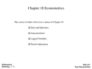
Chapter 18 Econometrics. This series of slides will cover a subset of Chapter 18 Data and Operators Autocorrelated Lagged Variables Partial Adjustment. Repeated Firm or Consumer Data. Time Structured Data - [y 1 , y 2 , …, y t , …, y T ] Error Structure - Not Gauss-Markov ( 2 I ).

Chapter 18 Econometrics
E N D
Presentation Transcript
Chapter 18 Econometrics • This series of slides will cover a subset of Chapter 18 • Data and Operators • Autocorrelated • Lagged Variables • Partial Adjustment
Repeated Firm or Consumer Data • Time Structured Data - [y1, y2, …, yt, …, yT] • Error Structure - Not Gauss-Markov (2I)
Backshift Operator The backshift operator, B, by definition produces xt-1 from xt Bxt = xt-1 Of course, one can also say BBxt = B2xt = xt-2 In general, Bjxt = xt-j
Autocorrelation Response Var Time Cov(yt, yt-1)?
Table for Autocorrelation y1 y2 y3 y4 y5 y6 y7 y8 y1 y2 y3 y4 y5 y6 y7 y8
Table for Autocorrelation y1 y2 y3 y4 y5 y6 y7 y8 y1 y2 y3 y4 y5 y6 y7 y8
Autocorrelated Error et = et-1 + t ~ N(0,2I)
Recursive Substitution in Time Series et = et-1 + t = (et-2 + t-1) + t = [(et-3 + t-2) + t-1] + t
Now We Leverage the Pattern et = [(et-3 + t-2) + t-1] + t = t + t-1 + 2t-2 + 3t-3 + … =
And Now Of course V(·) V(et) = E[et - E(et)]2 V(et) = E[et2] The previous slide showed that E(et) = 0
A Big Mess, Right? V(et) = E(et2) = (1 + 2 + 4 + …)2 Uh-oh… an infinite series…
Let’s Define the Infinite Series “s” s = 1 + 2 + 4 + 8 + … 2s = 2 + 4 + 8 + 16 + … What is the difference between the first and second lines? s - 2s = 1
Putting It Together Since
Applying the Same Logic to the Covariances For any pair of errors one time unit apart we have and in general
Instead of the Gauss-Markov Assumption (2I) we have V(e) = So how do we estimate now?
Lagged Independent Variables Consumer behavior and attitude do not immediately change: yt = 0 + xt-11 + et Or more generally: yt = 0 + xt-11 + xt-22 + ··· + et
Koyck’s Scheme Koyck started with the infinite sequence yt = xt0 + xt-11 + xt-22 + ··· + et and assumed that the values are all of the same sign
i i i s s s 0 0 0 i i i Lagged effects can take on many forms: Koyck (and others) have come up with ways of estimating different shaped impacts (1) assuming that only s lag positions really matter, and that (2) the impact of x on y takes on some sort of curved pattern as above
Further Assumptions • How many lags matter? In other words, how far back do we really need to go? Call that s. • Can we express the impact of those s lags with an even fewer number of unknowns. Any pattern can be approximated with a polynomial of degree r s (Almon’s Scheme). In Koyck’s Scheme, we will use a geometric rather than polynomial pattern.
We Rewrite the Model Slightly where wi 0 for i = 0, 1, 2, ···, and
Bring in the Backshift Operator and Assume a Geometric Pattern for the wi Now we assume that wi = (1 - )i 0 < < 1
Given Those Assumptions Anyone care to say how we got to this fraction?
Adaptive Adjustment Define as the expected level of x (prices, availability, quality, outcome)… So consumer behavior should look like
Updating Process Expectations are updated by a fraction of the discrepancy between the current observation and the previous expectation
Redefine in Terms of a New Parameter Define = 1 - so that
Back to the Model for yt We end up at the same place as slide 25