Download
1 / 20
220 likes | 558 Views
Strategic Capacity Planning. Strategic Capacity Planning. What is Capacity refers to an upper limit or ceiling on the load that an operating unit (plant, department, machine, stores and etc) can handle.

E N D
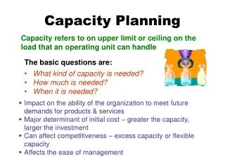
Strategic Capacity Planning • What is Capacity refers to an upper limit or ceiling on the load that an operating unit (plant, department, machine, stores and etc) can handle. • Goal of Strategic capacity planning is to achieve a match between long term supply capabilities and predicted level of long term demand to supports the firm’s long term competitive strategy.
Basic questions in capacity handling • What kind of capacity is needed? • Depends on product/services that management intend to provide. 2. How much is needed? • The volume and certainty of anticipated demand • Strategic objectives in terms of growth, customer service and competitions • The cost of expansion and operation • Time Dimension of Capacity: • Long Range • Intermediate Range • Short Range
Basic questions in capacity handling 3. When is it needed? • Capacity lead strategy • Capacity lag strategy • Average capacity strategy
Capacity Panning Concept • Capacity Utilization Ratio revels how close a firm to its best operating point : • Capacity used -rate of output actually achieved • Best operating level -capacity for which the process was designed and thus is the volume at which average unit cost is minimized.
Designing Measuring Capacity Design capacity = 50 trucks/day Effective capacity = 40 trucks/day Actual output = 36 units/day Actual output = 36 units/day Efficiency = = 90% Effective capacity 40 units/ day Utilization = Actual output = 36 units/day = 72% Design capacity 50 units/day Effective capacity-affected by periodic maintenance, lunch break, problem in scheduling and operation, imbalance line etc Actual capacity affected by breakdown, absenteeism, shortage and poor quality of raw material etc
Capacity Panning Concept • Economies of Scale : as a plant gets larger and volume increases the average cost per unit of output drops. Reasons for economies of scale are: • Reducing the fix cost per unit • Construction costs increases at a decreasing rate • Processing costs decrease as output rate increases because operations become more standard. • Diseconomies of Scale : when higher level of output cost more per unit to produce. Reasons for diseconomies of scale are: • Distribution costs increases due to traffic congestion and shipping from one large facility to several smaller ones. • Complexity increases costs, command and communication become more problem. • Inflexibility can be issue • Increased bureaucracy, slowing decision making and late approval
Capacity Panning Concept • The Experience Curve -As plants produce more products, they gain experience in the best production methods and reduce their costs per unit • Capacity Focus -The concept of the focused factory holds that production facilities work best when they focus on a fairly limited set of production objectives. • Plants Within Plants (PWP) extend focus concept to find best operating level • Capacity Flexibility – Ability to increase or decrease production levels, or to shift production capacity from one product or service to another. • Flexible plants, Flexible process, Flexible workers
Determining Capacity Requirements 1. Forecast sales within each individual product line 2. Calculate equipment and labor requirements to meet the forecasts 3. Project equipment and labor availability over the planning horizon • Capacity Cushion – is an amount of capacity in excess of expected demand. This may be positive or negative. • Positive Capacity Cushion - when a firm’s design capacity is more than capacity required to meet its demand • Negative Capacity Cushion - when a firm’s design capacity is less than capacity required to meet its demand
Example of Capacity Requirements A manufacturer produces two lines of mustard, FancyFine and Generic line. Each is sold in small and family-size plastic bottles. The following table shows forecast demand for the next four years.
Example of Capacity Requirements (Continued) : Equipment and Labor Requirements • Three 100,000 units-per-year machines are available for small-bottle production. Two operators required per machine. • Two 120,000 units-per-year machines are available for family-sized-bottle production. Three operators required per machine.
At 1 machine for 100,000, it takes 1.5 machines for 150,000 150,000/300,000=50% At 2 operators for 100,000, it takes 3 operators for 150,000 Question: What are the Year 1 values for capacity, machine, and labor? • The McGraw-Hill Companies, Inc., 2004
Question: What are the values for columns 2, 3 and 4 in the table below? 56.67% 1.70 3.40 66.67% 2.00 4.00 80.00% 2.40 4.80 58.33% 1.17 3.50 70.83% 1.42 4.25 83.33% 1.67 5.00 • The McGraw-Hill Companies, Inc., 2004
Example of a Decision Tree Problem A glass factory specializing in crystal is experiencing a substantial backlog, and the firm's management is considering three courses of action: A) Arrange for subcontracting B) Construct new facilities C) Do nothing (no change) The correct choice depends largely upon demand, which may be low, medium, or high. By consensus, management estimates the respective demand probabilities as 0.1, 0.5, and 0.4.
Example of a Decision Tree Problem (Continued): The Payoff Table The management also estimates the profits when choosing from the three alternatives (A, B, and C) under the differing probable levels of demand. These profits, in thousands of Taka are presented in the table below:
A B C Example of a Decision Tree Problem (Continued): Step 1. We start by drawing the three decisions
Tk 90 High demand (0.4) Tk 50 Medium demand (0.5) Tk 10 Low demand (0.1) A Tk 200 High demand (0.4) Tk 25 B Medium demand (0.5) - Tk 120 Low demand (0.1) C Tk 60 High demand (0.4) Tk 40 Medium demand (0.5) Tk 20 Low demand (0.1) Example of Decision Tree Problem (Continued): Step 2. Add our possible states of nature, probabilities, and payoffs
High demand (0.4) Medium demand (0.5) Low demand (0.1) Example of Decision Tree Problem (Continued): Step 3. Determine the expected value of each decision $90 $50 $62 $10 A EVA=0.4(90)+0.5(50)+0.1(10)=$62
$90 High demand (0.4) $50 Medium demand (0.5) $10 Low demand (0.1) A $200 High demand (0.4) $25 B Medium demand (0.5) -$120 Low demand (0.1) C $60 High demand (0.4) $40 Medium demand (0.5) $20 Low demand (0.1) Example of Decision Tree Problem Step 4. Make decision Tk 62 Tk 82 $80.5 Tk 46 Alternative B generates the greatest expected profit, so our choice is B or to construct a new facility
Planning Service Capacity vs. Manufacturing Capacity • Time: Goods can not be stored for later use and capacity must be available to provide a service when it is needed • Location: Service goods must be at the customer demand point and capacity must be located near the customer • Volatility of Demand: Much greater than in manufacturing Capacity Utilization & Service Quality • Best operating point is near 70% of capacity • From 70% to 100% of service capacity, what do you think happens to service quality?