Download
1 / 30

E N D
1. Chaos Mappings
2. Flows vs. Maps System of ordinary first-order differential equations:
where t = independent variable
xi � x1, x2, . . . , xn.
example of a flow
3. Flows Flow � gives rise to continuous evolution of �field lines� in the n-dimensional space (or �phase space�)
If the volume in space remains constant with time, the flow is conservative.
If the volume in space decreases with time, the flow is dissipative.
A dampening effect in dynamics like friction
4. Flows The first system of equations can be written in column vector form:
5. Lorenz Equations Chaotic effects arises when
At least one of the functions fi contains a nonlinear term (e.g., x12, x12x2, x1x23)
The dimension of the system of equations is 3 or greater
s, r, and b are all constants
Lorenz attractor � when s = 10, b = 8/3, and r = 28
6. Dynamic Systems as Maps XN+1 = G(XN), N = 1, 2, . . .
can be defined by the column vectors
where N labels the Nth iteration of the map
7. Dynamic Systems as Maps A map can be generated from a flow by taking:
X(t), X(t + t), X(t + 2t), . . . X0, X1, X2, . . .
Condition for chaos in mappings
Must contain at least one nonlinear term
8. Flows vs. Maps
9. Simple Maps The logistic map
The H�non attractor
Chaos esth�tique
The Standard Map
10. The Logistic Map Xn+1 = axn(1-xn)
At iteration 1000
1.0 � below this value the population cannot survive
2.0 � oscillatory approach to the asymptotic value
3.0 � �period� of the population doubles
3.45 � �something else happens�
11. The Logistic Map Adding iteration 1001
At around 3.57 � chaos emerges
Chaos does not necessarily imply disorder
Chaos is the �randomness� in predicting the next iteration
12. The Logistic Map Adding iteration 1003
Period quadruples at 3.449499
13. The Logistic Map 256 iterations after i1000
3.544090 � period of 8
3.564407 � period of 16
3.568759 � period of 32
3.569692 � period of 64
3.569946 � period doubling ends
14. The Logistic Map One of the branches is a small replication of the entire function
�Self similarity� across scales
15. The Logistic Map Y range = 0.489 � 0.52
X range = 3.625 � 3.638
Box: 3.6339 � 3.6342
16. The Logistic Map Y range = 0.491 � 0.501
Box = 3.634042 � 3.634052
17. The Logistic Map Y range = 0.499621 � 0.50015
X range = 3.63404761 � 3.63404998
Magnification nearly 1 million times that of the first chaos mapping
18. The Logistic Map ~ 3.569946 � period doubling region ends and chaos begins
3.828427 � small period tripling window opens up
~ 3.855 � period tripling cascade ends and chaos resumes
~ 4.0 chaos reigns!!!
19. The Logistic Map Both periodicity and chaos in this picture
3.828427 � small period tripling window opens up
~ 3.855 � period tripling cascade ends and chaos resumes
20. The H�non Attractor 2-D map given by the equations:
xn+1 = yn + 1 � axn2
yn+1 = Bxn
General form of the attractor does not depend on initial x and y values
21. The H�non Attractor
22. The H�non Attractor Data generated through C++
Rendered with POVray
24bit undersampled 640x480 image
10 � 12 hours to render
http://www.ph.utexas.edu/~morrow/Henon/henon.html
23. The Chaos Esth�tique 2-D mapping for modeling the dynamics of a particle accelerator
xn+1 = yn + f(xn)
yn+1 = -bxn + f(xn+1)
where a and b are constants and
f(x) = ax + [2(1 � a)x2 / (1 + x2)]
24. Conservative Mapping
25. Dissipative Mapping
26. The Standard Map 2-D map to model accelerator dynamics
qn+1 = qn + pn+1
pn+1 = pn + (k/2p) sin(2pqn)
for small values of k there is no chaos
for values of k above ~ 4 chaos reigns
the onset of widespread chaotic behavior occurs ~ 0.9716
27. The Standard Map closed loops � stable regions with fixed or periodic points at the centers
hazy regions � unstable and chaotic
28. The Standard Map
29. References D. Gulick, �Encounters with Chaos� (McGraw Hill, Inc., New York, 1992), pp. 127-186, 195-220, 240-285
P. Berge, Y. Pomeau, and C. Vidal, �Order Within Chaos; Towards a Deterministic Approach to Turbulence� (John Wiley & Sons, New York, 1984), pp. 111-144, 301-324.
R. Devaney, �A First Course in Chaotic Dynamical Systems� (Addison-Wesley Publishing Company, Inc., New York, 1992), pp. 154-163.
H. Lauwerier, �Fractals: Endlessly Repeating Geometrical Figures� (Princeton University Press, Princeton, N.J., 1991), p. 136.
M. Tabor, �Chaos and Integrability in Nonlinear Dynamics, An Introduction� (John Wiley & Sons, New York, 1989), pp. 134-167.
K. T. R. Davies and M. Baranger, to be published.
30. Web References Exploring the Logistic Map � M. Casco Associates
Strange attractors � Henon, etc.
Standard Map - Cirikov-Taylor map
Heun attractor program in BASIC