
מיקרוסקופיה פלואורסנטית
מיקרוסקופיה פלואורסנטית. Contrasting techniques - a reminder…. Brightfield - absorption Darkfield - scattering Phase Contrast - phase interference Polarization Contrast - polarization Differential Interference Contrast (DIC) - polarization + phase interference
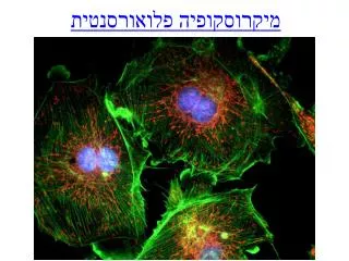

מיקרוסקופיה פלואורסנטית
E N D
Presentation Transcript
Contrasting techniques - a reminder… • Brightfield - absorption • Darkfield - scattering • Phase Contrast - phase interference • Polarization Contrast - polarization • Differential Interference Contrast (DIC) - polarization + phase interference • Fluorescence Contrast - fluorescence
שיטות להגברת ניגודיות Bright-field DIC חוב מהשיעור הקודם Phase-contrast Dark-field
Fluorescence techniques • Standard techniques: wide-field confocal 2-photon • Special applications: FRET FLIM FRAP Photoactivation TIRF
Excited state Ground state Fluorescence excitation shorter wavelength, higher energy emission longer wavelength, less energy Stoke’s shift
Fluorophores(Fluorochromes, chromophores) • Special molecular structure • Aromatic systems (Pi-systems) and metal complexes (with transition metals) • characteristic excitation and emission spectra
Filters How can we separate light with specific wavelength from the rest of the light?
Filter nomenclature • Excitation filters: x • Emission filters: m • Beamsplitter (dichroic mirror): bs, dc, FT • 480/30 = the center wavelength is at 480nm; full bandwidth is 30 [ = +/- 15] • BP = bandpass, light within the given range of wavelengths passes through (BP 450-490) • LP = indicates a longpass filter which transmits wavelengths longer than the shown number and blocks shorter wavelengths (LP 500) • SP = indicates a shortpass filter which transmits wavelengths shorter than the shown number, and blocks longer wavelengths
Filters Multiple Band-Pass Filters
Basic design of epi fluorescence Objective acts as condenser; excitation light reflected away from eyes
The cube • Excitation/emission spectra always a bit overlapping • filterblock has to separate them • Exitation filter • Dichroic mirror • (beamsplitter) • Emission filter
excitation and emission spectra of EGFP (green) and Cy5 (blue) excitation and emission spectra of EGFP (green) and Cy2 (blue) No filter can separate these wavelengths! Excitation / emission
Where to check spectra? You can plot and compare spectra and check spectra compatibility for many fluorophores using the following Spectra Viewers. Invitrogen Data Base BD Fluorescence Spectrum Viewer University of Arizona Data Base Fluorescent Probe Excitation Efficiency(Olympus jave tutorial) Choosing Fluorophore Combinations for Confocal Microscopy(Olympus java tutorial)
Photobleaching • Photobleaching - When a fluorophore permanently loses the ability to fluoresce due to photon-induced chemical damage and covalent modification.
Photobleaching • At low excitation intensities, pb occurs but at lower rate. • Bleaching is often photodynamic - involves light and oxygen. • Singlet oxygen has a lifetime of ~1 µs and a diffusion coefficient ~10-5 cm2/s. Therefore, potential photodamage radius is ~50 nm.
Standard techniques • wide-field • Confocal • Spinning disk confocal • 2-photon
Wide-field fluorescence • reflected light method • Multiple wavelength source (polychromatic, i.e. mercury lamp) • Illumination of whole sample
Wide-field vs confocal Wide-field image confocal image Molecular probes test slide Nr 4, mouse intestine
Point illumination Widefield Illumination Point Illumination
Light sources for point illumination Excitation light must be focused to adiffraction limited spot Excitation light Could be done with an arc lampand pinhole – but very inefficient Enter the laser: Perfectly collimated and high power Objective lens Sample
Point illumination Fluorescence Illumination of a single point Camera Tube lens Excitation light Emission light Objective lens Sample Problem – fluorescence is emitted along entire illuminated cone, not just at focus
The confocal microscope Detector Pinhole Tube lens Excitation light Emission light Objective lens Sample
The confocal microscope • method to get rid of the out of focus light less blur • whole sample illuminated (by scanning single wavelength laser) • only light from the focal plane is passing through the pinhole to the detector
Scanning Changing entrance angle of illumination moves illumination spot on sample Objective lens The emission spot moves, so we have to make sure pinhole is coincident with it Sample
Improved PSF and pinhole size • Why can’t it be as small as possible? • Reduced number of photons that arrive at the detector from the specimen may lead to a reduced signal-to-noise ratio. • Raising the intensity of the excitation light can damage the specimen. • Optical sectioning does not improve considerably with the pinhole size below a limit that approximates the radius of the first zero of the Airy disk. PSF for the focal plane and planes parallel to it: (a) conventional diffraction pattern (b) Confocal case.
How big should your pinhole be? Width of point spread function at pinhole = Airy disk diameter × magnification of lens = 1 Airy unit= resolution of lens × magnification of lens × 2 100x / 1.4 NA: resolution = 220nm, so 1 Airy unit = 44 mm 40x / 1.3 NA: resolution = 235nm, so 1 Airy unit = 19 mm 20x / 0.75 NA: resolution = 407nm, so 1 Airy unit = 16 mm 10x / 0.45 NA: resolution = 678nm, so 1 Airy unit = 14 mm
How big should your pinhole be? A pinhole of 1 airy unit (AU) gives the best signal/noise. A pinhole of 0.5 airy units (AU) will often improve resolution IF THE SIGNAL IS STRONG.
Confocal Use: • to reduce blur in the picture high contrast fluorescence pictures (low background) • optical sectioning (without cutting); 3D reassembly possible Careful: increasing image size (more pixels) does not mean that the objective can resolve the same!!! (resolution determined by NA, a property of the objective)
Spinning Disk Fast – multiple points are illuminated at once Photon efficient – high QE of CCD Gentler on live samples – usually lower laser power Fixed pinhole Small field of view (usually) Crosstalk through adjacent pinholes limits sample thickness
Relative Sensitivity Widefield 100 Spinning-Disk Confocal 25 Laser-scanning Confocal 1 See Murray JM et al, J. Microscopy 2007 vol. 228 p390-405
Excited state Ground state 2-photon microscopy Excitation: long wavelength (low energy) Each photon gives ½ the required energy Emission: shorter wavelength (higher energy) than excitation
2-photon microscopy • Use of lower energy light to excite the sample (higher wavelength) 1-photon: 488nm 2-photon: 843nm Advantages: • IR light penetrates deeper into the tissue than shorter wavelength • 2-photon excitation only occurs at the focal plane less bleaching above and below the section Use for deep tissue imaging
Special applications: • FRET and FLIM • FRAP/FLIP and photoactivation • TIRF
Exited state Exited state Exited state Ground state Ground state Ground state FRET (FluorescenceResonanceEnergyTransfer) • method to investigate molecular interactions • Principle: a close acceptor molecule can take the excitation energy from the donor (distance 1-10 nm) FRET situation: Excitation of the donor (GFP) but emission comes from the acceptor (RFP) No FRET Energy transfer, no emission! Donor (GFP) Acceptor (RFP)
Both Acceptor and Donor are fluorescent The Donor is excited and its emission excites the Acceptor Ex(D) Em(A) Em(D) Ex(A) FRET
FRET is a competing process for the disposition of the energy of a photo excited electron. Donor emission decreases Donor lifetime decreases Acceptor emission increases FRET
Energy transfer efficiency Depends on: Donor emission and acceptor absorption spectra, relative orientation of D and A FRET
FRET ways to measure: • Acceptor emission Detect the emission of the acceptor after excitation of the donor, e.g. excite GFP with 488 but detect RFP at 610 (GFP emission at 520) • Donor emission after acceptor bleachingtake image of donor, then bleach acceptor (with acceptor excitation wavelength - RFP:580nm), take another image of donor should be brighter!
∆t=lifetime FLIM(Fluorescence Lifetime Imaging Microscopy) • measures the lifetime of the excited state (delay between excitation and emission) • every fluorophore has a unique natural lifetime • lifetime can be changed by the environment, such as: • Ion concentration • Oxygen concentration • pH • Protein-protein interactions
FLIM - advantages 1/e 1 2 • In this method we measure the lifetime of the excited state and not the fluorescence intensity, therefore: • We can separate fluorophores with similar spectra. • We minimize the effect of photon scattering in thick layers of sample. lifetime = ½ of all electrons are fallen back
FLIM - Measurement approaches Time gates • Frequency domain • Modulated excitation • Lock-in detect emission phase • Time domain (pulsed exc.) • Gated intensifier • Photon inefficient • Time-correlated • single photon counting • Very efficient • one photon per pulse slow