Remote sensing magnetic reconnection in the magnetosphere.

1. Remote sensing magnetic reconnection in the magnetosphere. Mervyn Freemanand the Magnetic Reconnection project team British Antarctic Survey, Cambridge www.antarctica.ac.uk/BAS_Science/Programmes/MRS/mrproject/index.html 17 August 2004 Magnetic Reconnection Theory Workshop, Cambridge

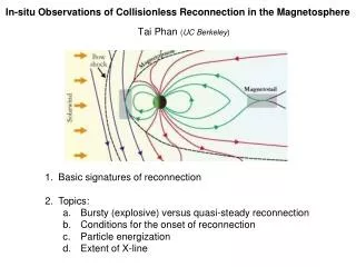
2. This talk • Geospace is the only natural environment in which reconnection can be sensed both • in-situ (local) • by spacecraft • remotely (local - global) • by instruments on earth • using dipole magnetic field as a lens • Explain ground-based radar signatures of reconnection • Show examples of reconnection studies and results.

3. Why remote sensing? • In-situ spacecraft observations • Direct but localised in time and space • Remote sensing • Indirect but continuous observations of regions across the MHD scales • When? • Continuous or intermittent? • Driven or spontaneous? • Where? • Anti-parallel or component reconnection? • Homogeneous or patchy?

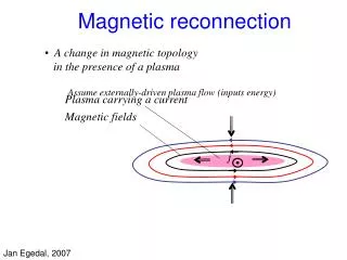
4. Principles of ground-based remote sensing • Reconnect magnetic field line with at least one footpoint • Reconnected magnetic field lines near separatrices communicate signatures to low altitude detectable from ground such that • separatrices can be identified • distinct magnetic topologies with different environments and/or • distinct separatrix surface signatures • reconnection rate can be estimated • from measurement of E x B plasma motion across separatrices

5. Solar example z • Separatrix between open and closed magnetic field lines identified by super-hot particles • Reconnection rate derived from • footpoint motion of separatrix, ubx • normal magnetic field Bzin photosphere • plasma velocity is zero in photosphere x ubx

6. Magnetosphere example • Separatrix between open and closed magnetic field lines identified by accelerated magnetosheath particles in cusp • Reconnection rate derived from • footpoint plasma velocity normal to separatrix, vx • footpoint motion of separatrix, ubx • normal magnetic field Bzin ionosphere • Similarly on nightside Earth Bz ubx vx

7. Radar remote sensing • Use Super Dual Auroral Network (SuperDARN) of HF radars • to identify separatrixand • to measure E x B velocity • 8 radars in northern hemisphere • 6 radars in southern hemisphere • more coming!

8. Halley X + South pole X geographic + magnetic Halley HF radar array • Electronically steered phased-array antennae • 16 log-periodic antennae give 16 possible beam azimuths • 75 ranges with 45 km spatial separation • Each beam sampled every 7 s • Full scan every 2 min

9. Target V a Vcosa Antenna irregularities 300 km B 500-1000 km HF radar measurement of E x B plasma motion • RAdio Detecting And Ranging • Radar signal is backscattered off target • Time delay measures range of target • Doppler shift measures line-of-sight velocity of target • Target is field-aligned electron density irregularities in F-region ionosphere (~300 km altitude) • created by plasma instabilities • backscatter HF radar waves where wave vector is refracted perpendicular to magnetic field • move at E x B drift velocity

10. SuperDARN velocity maps Sun • Combine line-of-sight velocity measurements into global convection map by spherical harmonic fit to data from different lines of sight, assuming incompressible flow, and using statistical model to fill gaps magnetic pole

11. Identification of open-closed separatrix • Reconnection in earth’s magnetosphere creates different plasma regions in magnetosphere and at magnetic footpoints in ionosphere • Identified by flux and energy of magnetic field-aligned particles “precipitating” to low altitude

12. ocb ocb Radar proxy for open-closed separatrix[Chisham and Freeman, Ann. Geophys., 21, 983, 2003; 22, 1187, 2004;Chisham et al., Geophys. Res. Lett., 31, L02804, 2004] • Compared spacecraft measurements of open-closed separatrix with contemporaneous and co-located radar measurements • Separatrix is co-located with a boundary in radar spectral width • measure of small-scale velocity structure • increases poleward of separatrix • Valid on both dayside and nightside (except 2-10 MLT)

13. Example 1: Reconnection for southward IMF[Pinnock et al., Ann. Geophys., 21, 1647, 2003] • Magnetopause reconnection X-line expected to be on equator • Phan et al. [Nature, 404, 848, 2000] report bi-directional reconnection jets centred on equator near dawn flank • steady southward interplanetary magnetic field • How long is X-line? • Is reconnection continuous or intermittent? • Driven or spontaneous?

14. - DMSP O Equator-S O Geotail SuperDARN remote sensing • Analyse SuperDARN data over Phan et al. interval • Convection consistent with standard 2-cell convection • Separatrix and E x B velocity measured continuously (2 min resolution) • over much of dayside magnetopause (9-16 MLT)

15. Equator-S Reconnection rate – spatial structure • Reconnection electric field shows stable large-scale structure • Reconnection signature seen at Equator-S footpoint (~0.5 mV/m) • Reconnection extends beyond dawn and dusk flanks on equator • Length >~ 38 RE

16. Reconnection rate – temporal structure • Reconnection is continuous during continuous IMF Bz < 0 • Some fluctuation • not clearly related to IMF driver

17. Example 2: Reconnection for northward IMF[Chisham et al., Ann. Geophys., in preparation, 2004] • Expect closure of open magnetic flux poleward of cusp • Reverse two-cell convection observed • Spatial extent of X-line footpoint much smaller than southward IMF

18. Reconnection rate – spatial structure • Reconnection electric field shows stable large-scale structure • Reconnection rate at magnetopause similar to southward IMF (~0.5 mV/m) • Reconnection footpoint maps poleward of cusp • Length <~ 10 RE

19. Reconnection rate – temporal structure • Reconnection is continuous during continuous IMF Bz > 0 • Some fluctuation • not clearly related to IMF driver • Global reconnection rate much smaller than for southward IMF • limited by X-line extent

20. Example 3: Reconnection for arbitrary IMF[Coleman et al., J. Geophys. Res., 2000; J. Geophys. Res., 2001; Chisham et al., J. Geophys. Res., 2002] • How do macroscopic magnetic fields and plasma flows control reconnection? • Where does reconnection occur? • Is it sub-solar? • slow flow • Is it anti-parallel? • high magnetic shear • Is there a critical experimental test? View from Sun of geomagnetic field (black) and interplanetary magnetic field (blue). Regions of 180 degree magnetic shear shown in red. Subsolar region of slow flow shown in green.

21. VA< V N S VA> V 2 hr merging gap December Solstice Bz< 0 | By |  | Bz | Stagnant Flow Anti-parallel reconnection test • Test if magnetic shear is most important factor controlling reconnection. • 2 reconnection sites on magnetopause with gap between them in winter hemisphere. • Stagnant flow in gap

22. As predicted, for Northern hemisphere midwinter, two regions of strong poleward flow either side of noon With stagnation and weaker equatorward flow at noon Critical test for reconnection location Observed convection at noon from SuperDARN • Reconnection preferentially occurs where magnetic fields are anti-parallel, irrespective of other conditions

23. Lockwood and Wild [1993] Transient reconnection • Transient and localised reconnection at the magnetopause has been associated with transient convection and aurora: • flux transfer events (FTEs) • flow channel events (FCEs) • poleward moving auroral forms (PMAFs) • Similarly for reconnection in the magnetotail: • bursty bulk flows (BBFs) • poleward boundary intensifications (PBIs) • Transients may transport majority of magnetic flux and energy. Neudegg et al. [1999]

24. Complex reconnection?[Abel and Freeman, J. Geophys. Res., 2002] • Similar distributions of waiting times for • Flux Transfer Events (solid, dotted) • Pulsed Ionospheric Flows (dash-dot) • Poleward Moving Auroral Forms (dashed) • No characteristic scale (power law) above minimum resolvable scale (2-3 min)? • Velocity fluctuations are self-similar on different temporal and spatial scales

25. SOC Reconnection? • Distributions of areas and durations of auroral bright spots are power law (scale-free) from kinetic to system scales [Uritsky et al., JGR, 2002; Borelov and Uritsky, private communication] • Could this be associated with multi-scale reconnection in the magnetotail? • Self-organisation of reconnection to critical state (SOC) [e.g., Chang, Phys. Plasmas, 1999] • cf SOC in the solar corona [Lu, Phys. Rev. Lett., 1995]

26. Conclusions • Magnetic reconnection is a universal phenomenon • Sun, stars, accretion disks, geospace, etc. • Geospace is the only natural environment in which reconnection can be observed both remotely (globally) and in-situ (locally). • Can address universal questions: • Remote sensing observations suggest that: • reconnection preferentially occurs where magnetic fields are anti-parallel, irrespective of other conditions • magnetopause reconnection is driven • reconnection may occur on many time and space scales with no characteristic scale