Download

1 / 14
140 likes | 257 Views
This study explores the use of hierarchical Bayesian models in pharmacokinetics, particularly when dealing with data collected at different levels of aggregation. It highlights the challenges of standard techniques that either oversimplify group population assumptions or disregard aggregate information. We present a Bayesian setup, introducing hyperpriors to account for the variability among different groups. Furthermore, we discuss optimal design methodologies for maximizing the efficacy of Monte Carlo experiments involving simulation of new patient data and estimation of parameters for pharmacological studies.

E N D
Pharmacokinetics Modeling Linas Mockus
Hierarchical Bayes • Hierarchical data is ubiquitous where measurement occurs at different levels of aggregation. • we collect measurements of students who attend certain school. • When this occurs, standard techniques either assume that these groups belong to entirely different populations or ignore the aggregate information entirely. • Hierarchical models provide a way of pooling the information for the disparate groups without assuming that they belong to precisely the same population.
Bayesian Setup • Suppose we have collected data about some random variable Y from m different groups with n observations for each group. • Let yij represent observation j from group i. • Suppose yij ~ f(i), where i is a vector of parameters for group i. • Further, i ~ f() may also be a vector • note, until this point this is just a standard Bayesian setup where we are assigning some prior distribution for the parameters that govern the distribution of y.
Bayesian Setup • Now we extend the model, and assume that the parameters 11, 12 that govern the distribution of the ’s are themselves random variables and assign a prior distribution to these variables as well: ~ f(a,b),where, is called the hyperprior. The parameters a,b,c,d for the hyperprior may be “known” and represent our prior beliefs about or, in theory, we can also assign a probability distribution for these quantities as well, and proceed to another layer of hierarchy.
Graphical Representation Hyperpriors for the full population Priors for each group Data
Effect of Grouping Grouping by genetic variation in renal drug transporters in API secretion in vivo
Effect of Grouping node mean sd FV.p 8.174E-6 9.18E-7 Ka.p 0.3996 0.0573 Ke.p 0.1371 0.01074 sigma 0.684 0.03178 node mean sd FV.p1 0.2861 0.09346 FV.p2 9.467E-6 1.844E-6 Ka.p1 1.16 0.1699 Ka.p2 0.3664 0.08707 Ke.p1 0.139 0.01527 Ke.p2 0.1403 0.01941 sigma 0.6856 0.03194
Effect of Grouping Homozygous for the common variant L503F Homozygous for the common allele 503L
Transit Compartment Model • No discontinuity as in lag model • Better description of the underlying physiology
Optimal Design • Optimal Design via Curve Fitting of Monte Carlo Experiments • Peter Muller and Giovanni Parmigiani • Maximize payoff function
Optimal Design • Payoff • Calculate posterior of θ • Generate M new patients • Simulate K concentrations for each new patient • Estimate θ’for each new patient using experimental and simulated data
VariationalBayes • Port • R • Matlab • pharmaHUB