Probability Theory and Measure
190 likes | 355 Views
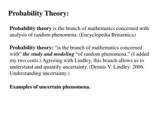
Probability Theory and Measure. Lecture III. Uniform Probability Measure. I think that Bieren’s discussion of the uniform probability measure provides a firm basis for the concept of probability measure .

Probability Theory and Measure
E N D
Presentation Transcript
Probability Theory and Measure Lecture III
Uniform Probability Measure • I think that Bieren’s discussion of the uniform probability measure provides a firm basis for the concept of probability measure. • First, we follow the conceptual discussion of placing ten balls numbered 0 through 9 into a container. • Next, we draw out an infinite sequence of balls out of the container, replacing the ball each time.
Taking each column, we can generate three random numbers {0.741483, 0.029645, 0.302204}. Note that each of these sequences are contained in the unit interval Ω=[0,1]. The primary point of the demonstration is that the number draw (xΩ=[0,1]) is a probability measure. • Taking x=0.741483 as the example, we want to prove that P([0,x=0.741483]) = 0.741483. To do this we want to work out the probability of drawing a number less than 0.741483. • As a starting point, what is the probability of drawing the first number in Table 1 less than 7, it is 7 ~{0,1,2,3,4,5,6}. Thus, without consider the second number, the probability of drawing a number less than 0.741483 is somewhat greater than 7/10.
Next, we consider drawing a second number given that the first number drawn is greater than or equal to 7. Now, we are interested in the scenario were the number drawn is equal to seven. This occurs 1/10 of the times. Note that the two scenarios are disjoint. If the first draw is less than seven, it is not equal to seven. Thus, we can rely on the summation rule of probabilities
Thus, the probability of drawing a number less than 0.74 is the sum of drawing the first number less than 7 and the second number less than 4 given that the first number drawn is 7. The probability of drawing the second number less than 4 is 4/10 ~ {0,1,2,3}. Given that the first number equal to 7 only occurs 1/10 of the time, the probability of the two events is
Continuing to iterate this process backward, we find that P([0,x=0.741483]) = 0.741483. Thus, for x Ωwe have P([0,x])=x. • A couple of things, first following our last lecture we have justified the use of probability measure defined on a σ-algebra. More concretely, we can define the unit interval as a special form of a σ-algebra called a Borel set. Second, the probability structure generated is a commonly used probability function, the uniform random variable, U[0,1].
Definition 1.5: The σ-algebra generated by the collection of all open intervals in R is called the Euclidean Borel field, denoted B, and its members are called Borel sets. • In this case, we have defined a = 0 and b= 1.
Also, note that for any This has the advantage of eliminating the lower end of the range. Specifically
Further, we have that as long as • In the Bieren’s formulation
This is probability measure is a special case of the Lebesgue measure.
Lebesgue Measure and LebesgueIntegral • Building on the Uniform Distribution example above, we next define the Lebesgue measure as a function λ that measures the length of the interval (a,b) on any Borel set B in R It is the total length of the Borel set taken from the outside.
Based on the Lebesgue measure, we can then define the Lebesgue integral based on the basic definition of the Reimann integral: • Replacing the interval of the summation, the Lebegue integral becomes:
Random Variables and Distributions • Now we have established the existence of a probability measure based on a specific form of σ-algebras called Borel fields. The question is then can we extend this rather specialized formulation to broader groups of random variables? Of course, or this would be a short class. • As a first step, let’s take the simple coin-toss example. In the case of a coin there are two possible outcomes (heads or tails). These outcomes completely specify the sample space.
To add a little structure, we construct a random variable Xthat can take on two values X = 0 or 1. • If X = 1 the coin toss resulted in a heads while if X = 0 the coin toss resulted in a tails. • Next, we define each outcome based on an event space ω:
The probability function is then defined by the random event ω. Defining ω as a uniform random variable from our original example one alternative would be to define the function as This definition results in the standard 50-50 result for a coin toss.
However, it admits more general formulations. For example, if we let The probability of heads becomes 40 percent.