Download
1 / 55
560 likes | 750 Views
Materials Management OPS 370. Independent Demand Inventory. Inventories and their Management. “ Inventories ” = ?. Types of Inventory. 1. Materials. Types of Inventory. 1. 2. 3. . Basic Inventory Management Issues And Decisions . Independent versus Dependent Demand.

E N D
Materials Management OPS 370 Independent Demand Inventory
Inventories and their Management “Inventories”= ?
Types of Inventory 1. Materials
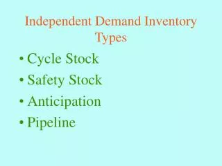
Types of Inventory 1. 2. 3.
Independent versusDependent Demand 1. Independent demand (This Chapter): 2. Dependent demand (Later):
Inventory Systems 1. An inventory system provides the structure and operating policies for maintaining and controlling goods to be stocked in inventory. 2. The system is responsible for ordering, tracking, and receiving goods. 3. There are two essential questions to answer that define a policy:
EOQ • 1. You want to review your inventory continually • 2. You want to replenish your inventory when the level falls below a minimum amount, and order the same Q each time • 3. Typical of a retail item, or a raw material item in a manufacturer
EOQ Assumptions • 1. For the Square Root Formula to Work Well: • A. Continuous review of the inventory position • B. Demand is known & constant …no safety stock is required • C. Lead time is known & constant • D. No quantity discounts are available • E. Ordering (or setup) costs are constant • F. All demand is satisfied (no shortages) • G. The order quantity arrives in a single shipment
Where the EOQ formula comes from: • Find the Q that minimizes the total annual inventory related costs: • Annual number of orders: N = D / Q • Annual Ordering Cost: S x (D / Q) • Average Inventory: Q / 2 2. Annual Carrying Cost: H x Q / 2
Annual cost ($) Order Quantity, Q How the costs behave:
Example:Papa Joe’s Pizza (Atlanta store) • Uses 18,000 pizza cartons / year • Ordering lead time is 1 month Decisions: • 1. How many cartons should Papa Joe order? i.e., Q • 2. When should Papa Joe order? R
Data: • Inventory carrying cost is $ .022 carton / year • Ordering cost is $10 / order
Reorder Point Q R 0 Lead Time
Q R OrderPlaced Demand duringlead time OrderReceived Stockout Variable Demand & Safety Stock
The Relationship BetweenSS, R, & L • R = enough stock to cover: • What you expectto happen during a lead time plus B. What mighthappen during the lead time C. R = dL + SS
EOQ with Discounts 1. Many companies offer discounted pricing for items that they sell. 2. Procedure: 3. Arrange the prices from lowest to highest. Starting with the lowest price, calculate the EOQ for each price until a feasible EOQ is found. A. If the first feasible EOQ is for the lowest price, this quantity is optimal and should be used. 4. If not, proceed until feasible EOQ found. A. If feasible EOQ found, check ALL breakpoints above the value of the feasible Q
EOQ w/ Quantity Discounts • Example • D = 16,000 boxes of gloves/year • S = $5/order • h = 0.25 (25% of cost) • C = cost per unit • $5.00 for 1 to 99 boxes • $4.00 for 100 to 499 boxes • $3.00 for 500+ boxes
EPQ • You want to review your inventory continually • You want to replenish your inventory when the level falls below a minimum amount, and order the same Q each time • Your replenishment does NOT occur all at once • Typical of a WIP item, typical of manufacturing
Illustration - - Papa Joe’s Pizza • Joe orders in batches of Q = 4000 cartons at a time • He uses a “low bid” vendor (cheap) • It takes about 1 month to get the order in • Due to limited staffing,only 1000 cartons can be made and sent to Joe each week How is the inventory build up different than the Base Case (EOQ scenario)?
And when should Papa Joe reorder his cartons ? R = Demand during the resupply lead time = d x L Reorder point is determined in the same way as for the EOQ policy
Other Types of Inventory Systems Variations on the basic types of continuous and periodic reviews: ABC Systems Bin Systems Can Order Systems Base Stock Systems The Newsvendor Problem
ABC Systems 1. ABCsystems: inventory systems that utilize some measure of importance to classify inventory items and allocate control efforts accordingly 2. They take advantage of what is commonly called the 80/20 rule, which holds that 20 percent of the items usually account for 80 percent of the value. A. Category A contains the most important items. B. Category B contains moderately important items. C. Category C contains the least important items.
ABC Systems 1. A items make up only 10 to 20 percent of the total number of items, yet account for 60 to 80 percent of annual dollar value. 2. C items account for 50 to 70 percent of the total number of items, yet account for only 10 to 20 percent of annual dollar value. 3. C items may well be of high importance, but because they account for relatively little annual inventory cost, it may be preferable to order them in large quantities and carry excess safety stock.
Example: Tee shirts are purchased in multiples of 10 for a charity event for $8 each. When sold during the event the selling price is $20. After the event their salvage value is just $2. From past events the organizers know the probability of selling different quantities of tee shirts within a range from 80 to 120: Customer Demand80 90 100 110 120 Prob. Of Occurrence .20 .25 .30 .15 .10 How many tee shirts should they buy and have on hand for the event?
Payoff Table: Setup Demand
Payoff Table: Cell Calculations Profit = Revenues – Costs + Salvage • Revenues = Selling Price (p)Amount Sold • Costs = Purchase Price (c) Purchase Qty • Salvage = Salvage Value (s)Amount Leftover Amount Sold = min (Demand, Purchase Qty) Amount Leftover = max (Purchase Qty – Demand, 0)
Payoff Table: Cell Calculations Have p = $20, c = $8, and s = $2. Compute Profit when Q = 90 and D = 110. Profit = [p Q]– [c Q] + [s 0] = (p – c) Q = Compute Profit when Q = 100 and D = 100. Profit = [p Q]– [c Q] + [s 0] = (p – c) Q = Compute Profit when Q = 110 and D = 80. Profit = [p D]– [c Q] + [s (Q – D)]=
Payoff Table Values Demand
Getting the Final Answer • 1. For Each Purchase Quantity: • A. Calculated the Expected Profit • 2. Choose Purchase Quantity With Highest Expected Profit. • 3. Expected Profit for a Purchase Quantity: • A. Multiply Each Payoff by Its Probability, Then Sum • 4. Example: