Introduction Application - ESP
Introduction Application - ESP. Electro Static Precipitator or Electrostatic air cleaner - ESP is used to filter and remove particles from a flowing gas - ESP contains rows of thin wires(electrodes) situated between large metal plates(collection electrodes)


Introduction Application - ESP
E N D
Presentation Transcript
IntroductionApplication - ESP • Electro Static Precipitator or Electrostatic air cleaner - ESP is used to filter and remove particles from a flowing gas - ESP contains rows of thin wires(electrodes) situated between large metal plates(collection electrodes) - High DC voltage between wires and plates - The particles are ionized by high voltage around the wires(cathode) and then attracted by the plates(anode) - The load in the ESP application shows capacitive behaviour Final Work Presentation
IntroductionDC/DC Power Converters • The need to convert a direct current(DC) voltage source from one voltage level to another • Linear conversion in compare to Switched Mode conversion • A DC/DC switching power converter stores the input energy temporarily and then releases that energy to the output at a different voltage level (this function motivates the switching property of the converter) • The storage may be in magnetic components, like inductors and transformers, or in capacitors • Different topologies has been introduced to fulfill our expectations, like Buck, Boost, Buck-Boost, Resonant power converter and etc. Final Work Presentation
IntroductionESP application and DC/DC power converters • The proper high load voltage is provided by a combination of a DC/DC power converter and a transformer • The resonant converter topology is chosen for the power converter • The switching is done by the four transistors (Transistors can be used as switches if they are saturated or cut-off) • Resonance circuit , switched system and rectifier • Switching frequency and resonance frequency • The load is connected in series to the resonance circuit Rectifier Final Work Presentation
IntroductionController and Observer • Controller and Observer in a resonant converter • Resonant phase plane controller • Control Signal: • States: Resonant current Resonant voltage Switched System(rectifier) W-1 - neg. conducting W0- not conducting W1 -pos. conducting Resonant circuit Final Work Presentation
Modeling of dynamic systems • Why modelling is needed? Analysis of system properties, controller design and observer design is based on the dynamic model of the system • The traditional differential equation form, ABCD form, A set of equations derived from physical law governing the system • The ABCD form is not global for non-linear systems and it eliminates the algebraic equations (some information of the system are lost) • Hamiltonian modelling is based on the energy properties of the system • Hamiltonian modeling DE-form and DAE-form • Power converter is a non-linear system due to existence of the switching transistors and rectifier, this motivates using Hamiltonian modelling Final Work Presentation
Hamiltonian Modelling is the Hamiltonian states is the energy storage function (Hamiltonian function) is a skew-symmetric matrix models how energy flows within the system, is a positive semi-definite symmetric dissipation matrix is a skew-symmetric control matrix *This model structure is used for modelling the converter* Final Work Presentation
Hamiltonian Modelling • Hamiltonian states, : charge on the capacitors, , and the magnetic flow in the inductors, • The energy function: • where and • The physical interpretation of Final Work Presentation
Hamiltonian modelling of the converter in DE-form • Decreasing the number of the states to four. magnetising inductance , , is high compared to the resonance inductance, making the magnetising current comparably small and possible to neglect. • Hamiltonian modelling in DE-form • Hamiltonian modelling is strongly related to the Graph Theory • Different block matrices in Hamiltonian DE-form must be defined according to graph theory • A Hamiltonian observer can be defined based on 4th order Hamiltonian model of the precess Final Work Presentation
4th order Hamiltonian model of the converter • Power converter is a switching system due to existence of the transistors and rectifier • The controller produce the proper function to switch the transistors • The rectifier has 3 possible conducting states: Positive conducting, Non-conducting and Negative conducting • Rectifier is acting in which subspase!? Ω1, positive conduction: Ω0, no conduction: Ω-1, negative conduction: Final Work Presentation
Modelling for subspace Ω0 • The graph in the subspase Ω0 • Spanning tree, tree branches and links • Component matrices, intermediate block matrices and the system block matrices are defined according to the graph theory The intermediate block matrices Final Work Presentation
Modelling for subspace Ω0 • The system block matrices The system equation: = + Final Work Presentation
Modelling for the subspaces Ω1 and Ω-1 In the subspaces Ω1 and Ω-1 the converter can be modelled by the graphs Different matrices must be defined for the upper configurations, the final result: where: Final Work Presentation
4th order global model • A global model is: • The 4th order global model of the converter system where • An Hamiltonian observer can be introduced based on the 4th order global model Final Work Presentation
Hamiltonian Observer • The structure of an Hamiltonian observer is given by • From the process model and the observer structure, the estimation error is given as , satisfies The error can be regarded as a . Hamiltonian system!! Final Work Presentation
Hamiltonian Observer • Error in the observer can be regarded as a Hamiltonian process with the Hamiltonian function(energy function): it is shown that (Hultgren, lenells 2004) : if • Note: The process is modelled by a 4th order Hamiltonian model and the observer is based on the 4th order Hamiltonian model of the process Final Work Presentation
Discretization of the observer • Controller creates control signal from the external signal (reference) and (estimation of the states) • Implementation of the controller: Analog or Digital • In the converter a phase plane feedback controller is used, this controller uses Resonance voltage and resonance current as feedbacks • The only measurment in this application is the resonance current • In discretization of the Hamiltonian observer, the sampling interval is very important (the error balance must be always negative) Final Work Presentation
Implementation in Matlab and Simulink Process Observer Final Work Presentation
Implementation in Matlab and Simulink Observer Model System Model Hamiltonian Observer Logic Final Work Presentation
Working Plane High Power vLN • Normalization of voltages and currents!? • Where is the operating point practically? • Does the observer works the same in all regions? • Where maximum error in state estimation happens? • Does the observer get unstable anywhere? • Which state has the most error? • How we can improve state estimation in the observer? • Different modelling? Optimal Sampling frequency? Result of simulation will answer the questions, hopefully correct! Low load current and high load voltage iLN High load current and low load voltage Final Work Presentation
High load current and Low load voltage, 10MHz sampling frequency High load current Square Wave Different subspaces! Spikes! High error! Final Work Presentation
High load current and Low load voltage, 30MHz sampling frequency Final Work Presentation
High load current and Low load voltage, 3MHz sampling frequency Error does not converge to zero! Final Work Presentation
Hamiltonian observer gain • How we can improve state estimation? Applying obser gain!? Changing the model!? • Applying an observer gain may improve state estimation but not always! • Lets have a look at trajectories: Final Work Presentation
Low load current and high load voltage, 30MHz sampling frequency Rectifier is operating mostly In the non-conducting mode Spikes are much lower Final Work Presentation
High load current and high load voltage (operating point), 10MHz sampling frequency • K=0 • K>0 Final Work Presentation
High load current and high load voltage (operating point), 30MHz sampling frequency • K=0 • K>0 Final Work Presentation
3rd order model of the process • If we have a lower order model of the system, implementation will be simpler and we have less calculation in the observer • By less calculation in the observer, we can discretize the observer with higher sampling frequency • Which state is candidate to be eliminated? • The load capacitance voltage is only slowly varying due to the high value of . During one conduction period of the rectifier the load voltage can be viewed as a constant voltage source, , in series with the voltage • The influence of the parallel capacitance, , is only significant when the rectifier is not conducting. In the case when the rectifier is conducting the parallel capacitance is connected in parallel with much larger load capacitance .During the periods when the rectifier is not conducting, the voltage of the parallel capacitance normally is commuting from to - or vice versa. The length of the non-conducting time periods is only significant when the load current is small. Final Work Presentation
3rd order model of the process • subspace Ω0 • subspaces Ω1 and Ω-1 System equation Global system equation Final Work Presentation
High load current and Low load voltage, 10MHz sampling frequency In this region, the rectifier is in the non-conducting mode for a short time K=0 K>0 Final Work Presentation
Low load current and High load voltage, 10MHz sampling frequency In this region, the rectifier is in the non-conducting mode for most of the time K=0 K>0 Final Work Presentation
High load current and high load voltage (operating point), 30MHz sampling frequency K=0 K>0 Final Work Presentation
Modelling of the system by considering resistance across the load capacitance The load in this industrial application shows obvious capacitive behaviour, but due to existence of corona current around the wires, the load shows resistivity behaviour too The modelling takes the same steps as we did for previous cases. First we define different subspaces , then we achieve the system equation according to Hamiltonian modelling and graph theory Final Work Presentation
Modelling of the system by considering resistance across the load capacitance subspace Ω0 = + subspaces Ω1 and Ω-1 where Final Work Presentation
Thank you for your attention! Final Work Presentation