Download
1 / 43
490 likes | 739 Views
ANOVA: Part I. Quick check for clarity. Variable 1 Sex: Male vs Female Variable 2 Class: Freshman vs Sophomore vs Junior vs Senior How many levels in Variable 1? Variable 2? Keep in mind: ‘Variable’ refers to what is being measured ‘Level’ refers to how many groups within the variable.

E N D
Quick check for clarity • Variable 1 • Sex: Male vs Female • Variable 2 • Class: Freshman vs Sophomore vs Junior vs Senior • How many levels in Variable 1? Variable 2? • Keep in mind: • ‘Variable’ refers to what is being measured • ‘Level’ refers to how many groups within the variable
Last week(s) • Since we’ve returned from break we’ve started analyzing data by comparing groups • More specifically, we’ve compared groups using one sample-, independent-, and paired samples t-tests • Also introduced the concepts of ‘degrees of freedom’ and ‘95% confidence intervals’ • Let’s take a moment to summarize when to use the different statistical tests we know…
Different statistical tests… • All tests are based on calculating a test statistic • Such as a t-score, Pearson’s r, etc… • Using the test statistic, the sample size, and number of groups (degrees of freedom) we estimate a p-value • While all of these tests are useful, they do have limits • Can’t have more than 1 independent variable • Except MLR • Can’t have more than 1 dependent variable • The dependent variable must be continuous
Where to now? • Moving forward, we’ll eliminate these restrictions: • ANOVA’s compare groups, and can be used with: • Multiple IV’s • IV’s with any number of levels • e.g., we can compare 5 variables with 3 levels each • MANOVA’s can be used with multiple DV’s • Chi-Square and Logistic Regression can make use of categorical DV’s (not continuous) • e.g., can predict heart attack vs no heart attack
Tonight’s topic • Tonight we’ll start discussing ANOVA • Like t-tests: • ANOVA’s are a family of statistical tests used to compare groups • ANalysis Of Variance • There are (basically) 3 types of ANOVA’s • Unlike t-tests, ANOVA’s can be used to compare two or more groups (levels) • More ‘flexibility’ and options than t-tests
Types of ANOVA’s • 1) One-Way ANOVA (basic, univariate) • Can compare one IV with any number of levels • i.e., compare mean GRE scores of ISU, IWU, and UI students • 2) Factorial ANOVA • Can do 1) above, plus… • Can use multiple IV’s (compare GRE by school and sex) • 3) Repeated Measures ANOVA • Can compare several groups (2 or more) in related subjects (paired groups, longitudinal data, etc…)
Back to the same dataset • I’m re-using the fitness test and academics dataset. • Dataset has information about FITNESSGRAM fitness tests and ISAT academic test scores in a group of adolescents • Again, I’m interested to know if academic success is related to health/fitness • We’ve seen how we can compare two groups using a t-test • But, if my question becomes more complicated, I’ll need to use ANOVA
Example • Is academic success related to physical fitness? • The ISAT test categorizes students into 3 groups: • Exceeding Standard (very good) • Meeting Standard (good enough) • Below Standard (not as good) • If academic success is related to fitness, I should be able to compare the fitness test results between these three groups • Do kids exceeding the standard have the highest ‘fitness’
Example • 3 Groups: Exceeds vs Meets vs Below Standard • I could use multiple t-tests to compare PACER laps between the three groups, right? • I’d need three: • t-test 1: Exceeds vs Meets • t-test 2: Exceeds vs Below • t-test 2: Meets vs Below • However, this violates a big statistical ‘law’. This approach is frowned upon for one big reason…
Family-Wise Error Rate • Using several t-tests instead of 1 ANOVA is not acceptable due to the Family-wise error rate • Also known as Experiment-wise error rate • Mathematically it can be complicated to explain, but let’s think of it like this: • If I set alpha at 0.05, that means I’m willing to accept a 5% risk of Type I error (random sampling error) • So, what happens if I complete 100 statistical tests on the same sample of people? • If each of my t-tests had an p-value of 0.05, odds are that I made a type I error 5 times out of 100
Even more simplistic explanation • Imagine I develop a pregnancy test and it is 95% accurate • Then, I have 100 women take the test. • I expect 95 tests will be correct – 5 tests will not • The theory is that it works the same way with random sampling error/Type I error. • If I’m 95% confident (alpha = 0.05) that I did not make a Type I error on 1 statistical test… • For every 100 tests, I can expect 5 to have Type I error
Family-wise Error • You can actually calculate this for yourself if you want to • 1 – Desired Confidence^Number of Tests = Chance of Type I error • Remember, our ‘desired confidence’ is 95%, or 0.95 • If we did 1 t-test, then: • 1 – 0.95^1 = 0.05 (notice, this is our normal chance of error) • 3 t-tests = 1 – 0.95^3 = 0.14, 14% chance of error • 13 t-tests = 1 – 0.95^13 = 0.49, 49% chance of error • The ‘goal’ of the ANOVA is to make multiple statistical comparisons but minimize risk of Family-wise error • By providing only one p-value
Back to the example • Instead of using 3 different t-tests (and 3 p-values), we use 1 ANOVA and create 1 p-value • For this example: • 1 IV Academic Success, 3 levels: Exceeds, Meets, Below • 1 DV PACER Laps (continuous variable) • HO: There is no difference in aerobic fitness between the three groups of academic success • HA: There is a difference in aerobic fitness between the three groups of academic success
Coding the IV • Here is how I coded my IV, academic success:
Degrees of Freedom • Recall ‘degrees of freedom’ is based on your number of groups and your number of subjects • For t-tests, we always have 2 levels so the df is always easy to calculate • # of Subjects - 2 • We always want to have the biggest df as possible (just like we want a large sample size) because it means we have a lower chance of Type I error
df in ANOVA’s • For ANOVA’s, we can have more than two groups, so pay close attention to your df – you will now have two • Degrees of Freedom 1 = # Groups – 1 • Degrees of Freedom 2 = # Subjects – # Groups • Df 1 is the ‘Between Groups’ df • It refers to making comparisons between our groups (ie, comparing Exceeds vs Meets vs Below) • Df 2 is the “Within Groups’ df • It refers to making comparisons between our subjects (ie, the total subjects ‘within’ all the groups)
Output from One-Way ANOVA • Here is your ANOVA output: • The sum of squares and mean square (ignore them) are used to calculate the F-ratio • Note df: • ‘Between Groups’ = 2 (3 groups – 1) • ‘Within Groups’ = 242 (245 subjects – 3 groups) N = 245
Output from One-Way ANOVA • Here is your ANOVA output: • We use df and the F-ratio to calculate the p-value • P = 0.006, which is less than 0.05, so we can say the test was statistically significant. Reject the null: • HA: There is a difference in aerobic fitness between the three groups of academic success N = 245
Output from One-Way ANOVA • P = 0.006, reject the null: • HA: There is a difference in aerobic fitness between the three groups of academic success • Do you have any other questions…? You should… • Notice, the ANOVA just says there is ‘a difference’ • We have no idea what groups are different… N = 245
Post-Hoc Tests • Our ANOVA indicates that at least one of our three groups is different from another one - but which one? • Exceeds vs Meets • Exceeds vs Below • Meets vs Below • We have to do a follow-up test, a Post-Hoc test, to determine where the significant difference(s) are • Post hoc just means ‘after this’ • ‘Mini’-tests used to find differences between groups AFTER a larger statistical test (like ANOVA)
WARNING with ANOVA’s • Please recognize: • ANOVA’s only provide you with half of the information • If your ANOVA is statistically significant – you HAVE TO continue to complete post-hoc tests • Run more tests to find the specific group differences • If your ANOVA is not statistically significant –you can STOP • None of the post hoc tests would be statistically significant (because the ANOVA just said they weren’t)
Post-Hoc tests • A large group of statistical tests that function like t-tests • They compare ONLY two groups, but they do it multiple times • SPSS aka ‘Pair-wise Comparisons’ • They are designed to avoid the family-wise error rate problem because they all ‘adjust’ the p-value based on the number of comparisons you make • i.e., they shrink your alpha level based on number of tests • As post-hoc tests and ANOVAs are strongly linked (you always run them together), SPSS accommodates this
Post-Hoc tests • LSD • Sidak • Scheffe • Duncan • They are pretty much all the same (for us) • The only one I want you to use in this class is Tukey • Perhaps the most commonly used post-hoc • Ignore every other post hoc test, unless told otherwise • Dunnett • SNK • Bonferroni • And more… • Several types of post-hoc tests you could use:
Post-Hoc tests • Let’s re-run our ANOVA, this time selecting a post-hoc test • If you don’t tell it to, SPSS will not automatically run it
More options • ‘Options’ can provide you with descriptive statistics
Descriptive Stats • The sample sizes, means, SD, and 95% CI for our three groups (dependent variable PACER Laps) individually and in total • Notice, this 95% CI is not for mean differences, but just the group mean
Output from One-Way ANOVA • This is the same output for the ANOVA we saw before, I just wanted to remind you of the p-value and decision • P = 0.006, reject the null: • HA: There is a difference in aerobic fitness between the three groups of academic success • Now, the post-hoc tests will tell us what groups
Post-Hoc: Tukey’s test, Multiple Comparisons • Now we have mean differences, p-values for each comparison, and 95% CI’s for the mean differences • Which groups are significantly different? • Remember, we are making 3 comparisons – but there are 6 tests results?
Post-Hoc: Tukey’s test, Multiple Comparisons • The ‘Exceeds’ group is significantly higher than the ‘Meets’ and ‘Below’ group (p = 0.034 and 0.008) • The ‘Meets’ group is NOT significantly different from the ‘Below’ group (p = 0.405)
Results in text • Results of the one-way ANOVA indicated that Pacer Laps were significantly different between Science Score groups (F(2, 242) = 5.17, p = 0.006). Tukey post-hoc comparisons revealed that the Exceeds group completed significantly more PACER laps than the ‘Meets’ group (p = 0.034) and the ‘Below’ group (p = 0.008). However, the ‘Meets’ group was not significantly different than the ‘Below’ group (p = 0.405). • If you wanted, you could also include the mean differences or means with 95% CI’s, but usually this is reported in a table since it can get complicated Questions on One-Way ANOVA?
A few more notes on ANOVA • SPSS also provides you with another output called ‘Homogenous Subsets’ • This feature is supposed to make it easy to see which groups are significantly different (or rather - which groups are the same, or homogenous):
A few more notes on ANOVA • SPSS also provides you with another output called ‘Homogenous Subsets’ • The problem with this feature is that it uses a slightly different method to calculate the p-values • It will sometimes give you different results! Ignore this! In our example, this output actually conflicts with what we found from the Tukey pairwise comparisons!
A few more notes on ANOVA • Statistical assumptions for the ANOVA are the same as those for the t-test! • 1) Normally distributed data • 2) Sample is representative of the population • 3) Homogeneity of variance • Unlike the t-test, we will not be using Levene’s test of Homogeneity – please ignore this as well
A few more notes on ANOVA • Our example compared 1 variable with 3 levels: • Exceeds, Meets, and Below • We had 3 post-hoc comparisons • Exceeds vs Meets; Exceeds vs Below; and Meets vs Below • Keep in mind what happens if you change the variable to have more levels: • For example, NHANES (a national health database) codes race as a 5-level variable: • Black, White, Mexican American, Other-Hispanic, Other • Assume we wanted to compare average blood pressure between these groups using a one-way ANOVA…
Multiple Comparisons Grow Quickly • Post-hoc tests would include several pair-wise comparisons: • Black, White, Mexican American, Other-Hispanic, Other • Black v White • Black v MexAm • Black v Oth-Hisp • Black v Other • White v MexAm • White v Oth-Hisp • White v Other • MexAm v Oth-Hisp • MexAm v Other • Oth-Hisp v Other This would be 10 comparisons Be mindful of how you organize your groups and variables, ANOVA’s can quickly get out of hand
Upcoming… • In-class activity • Homework: • Cronk complete 6.5 • Holcomb Exercises 49, 50, and 53 (on 95% CI’s) • More ANOVA next week • Factorial ANOVA!