Download
1 / 59
610 likes | 823 Views
Computing the shortest path on a polyhedral surface. Presented by: Liu Gang 2008.9.25. Overview of Presentation. Introduction Related works Dijkstra’s Algorithm Fast Marching Method Results. Introduction. Motivation.

E N D
Computing the shortest path on a polyhedral surface Presented by: Liu Gang 2008.9.25
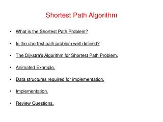
Overview of Presentation • Introduction • Related works • Dijkstra’s Algorithm • Fast Marching Method • Results
Motivation • Computing the shortest path between two points s and t on a polyhedral surface S is a basic and natural problem • From the viewpoint of application: • Robotics, geographic information systems and navigation • Establishing a surface distance metric
Related works Exact globally shortest path algorithms • Shair and Schorr (1986) On shortest paths in polyhedral spaces. O(n3logn) • Mount (1984) On finding shortest paths on convex polyhedral. O(n2logn) • Mitchell, Mount and Papadimitriou (MMP)(1987) The discrete geodesic problem. O(n2logn) • Chen and Han(1990) shortest paths on a polyhedron. O(n2) Approximate shortest path algorithms • Sethian J.A (1996) A Fast Marching Level Set Method for Monotonically Advancing Fronts. O(nlogn) • Kimmel and Sethian(1998) Computing geodesic paths on manifolds.O(nlogn) • Xin Shi-Qing and Wang Guo-Jin(2007) Efficiently determining a locally exact shortest path on polyhedral surface.O(nlogn)
Related works Exact globally shortest path algorithms • Shair and Schorr (1986) On shortest paths in polyhedral spaces. O(n3logn) • Mount (1984) On finding shortest paths on convex polyhedral. O(n2logn) • Mitchell, Mount and Papadimitriou (MMP)(1987) The discrete geodesic problem. O(n2logn) • Chen and Han(1990) shortest paths on a polyhedron. O(n2) Approximate shortest path algorithms • Sethian J.A (1996) A Fast Marching Level Set Method for Monotonically Advancing Fronts. O(nlogn) • Kimmel and Sethian(1998) Computing geodesic paths on manifolds.O(nlogn) • Xin Shi-Qing and Wang Guo-Jin(2007) Efficiently determining a locally exact shortest path on polyhedral surface.O(nlogn) Dijkstra's algorithm Fast Marching Methods(FMM)
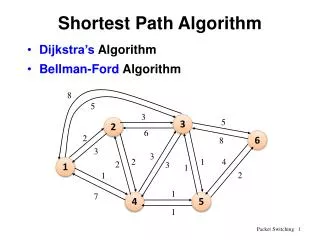
Dijkstra's Shortest Path Algorithm • Find shortest path from s to t. 2 24 3 9 s 18 14 6 2 6 4 19 30 11 5 15 5 6 16 20 t 7 44
Dijkstra's Shortest Path Algorithm 2 24 3 0 9 s 18 14 6 2 6 4 19 30 11 5 15 5 6 16 20 t 7 44 distance label
Dijkstra's Shortest Path Algorithm delmin 2 24 3 0 9 s 18 14 6 2 6 4 19 30 11 5 15 5 6 16 20 t 7 44 distance label
Dijkstra's Shortest Path Algorithm decrease key 9 X 2 24 3 0 9 s 18 14 X 14 6 2 6 4 19 30 11 5 15 5 6 16 20 t 7 44 distance label 15 X
Dijkstra's Shortest Path Algorithm delmin (0,9) X 2 24 3 0 9 s 18 14 X 14 6 2 6 4 19 30 11 5 15 5 6 16 20 t 7 44 distance label 15 X
Dijkstra's Shortest Path Algorithm (0,9) X 2 24 3 0 9 s 18 14 X 14 6 2 6 4 19 30 11 5 15 5 6 16 20 t 7 44 15 X
Dijkstra's Shortest Path Algorithm decrease key 33 X (0,9) X 2 24 3 0 9 s 18 14 X 14 6 2 6 4 19 30 11 5 15 5 6 16 20 t 7 44 15 X
Dijkstra's Shortest Path Algorithm 33 X (0,9) X 2 24 3 0 9 delmin s 18 (0,14) X 14 6 2 6 4 19 30 11 5 15 5 6 16 20 t 7 44 15 X
Dijkstra's Shortest Path Algorithm 32 33 X X (0,9) X 2 24 3 0 9 s 18 (0,14) X 14 6 2 6 44 4 X 19 30 11 5 15 5 6 16 20 t 7 44 15 X
Dijkstra's Shortest Path Algorithm 32 33 X X 9 X 2 24 3 0 9 s 18 (0,14) X 14 6 2 6 44 4 X 19 30 11 5 15 5 6 16 20 t 7 44 delmin 15 X
Dijkstra's Shortest Path Algorithm 32 33 X X (0,9) X 2 24 3 0 9 s 18 (0,14) X 14 6 2 6 35 44 X 4 X 19 30 11 5 15 5 6 16 20 t 7 44 59 X (0,15) X
Dijkstra's Shortest Path Algorithm delmin (6,32) 33 X X 9 X 2 24 3 0 9 s 18 14 X 14 6 2 6 35 44 X 4 X 19 30 11 5 15 5 6 16 20 t 7 44 59 X 15 X
Dijkstra's Shortest Path Algorithm (6,32) 33 X X (0,9) X 2 24 3 0 9 s 18 (0,14) X 14 6 2 6 35 44 X X 4 X 19 30 11 5 15 5 (3,34) 6 16 20 t 7 44 51 59 X X (0,15) X
Dijkstra's Shortest Path Algorithm (6,32) 33 X X (0,9) X 2 24 3 0 9 s 18 (0,14) X 14 6 (3,34) 2 6 35 44 X X 4 X 19 30 11 5 15 5 6 16 delmin 20 t 7 44 51 59 X X (0,15) X
Dijkstra's Shortest Path Algorithm (6,32) 33 X X (0,9) X 2 24 3 0 9 s 18 (0,14) X 14 6 2 6 45 35 X 44 X X 4 X 19 30 (3,34) 11 5 15 5 6 16 20 t 7 44 50 51 59 X X X (0,15) X
Dijkstra's Shortest Path Algorithm (6,32) 33 X X (0,9) X 2 24 3 0 9 s 18 (0,14) X 14 6 (3,34) 2 6 (5, 45) 35 X 44 X X 4 X 19 30 11 5 delmin 15 5 6 16 20 t 7 44 50 51 59 X X X (0,15) X
Dijkstra's Shortest Path Algorithm (6,32) 33 X X (0,9) X 2 24 3 0 9 s 18 (0,14) X 14 6 (6,34) 2 6 (5,45) 35 X 44 X X 4 X 19 30 11 5 15 5 6 16 20 t 7 44 50 51 59 X X X (0,15) X
Dijkstra's Shortest Path Algorithm (6,32) 33 X X (0,9) X 2 24 3 0 9 s 18 (0,14) X 14 6 (3,34) 2 6 (5,45) 35 X 44 X X 4 X 19 30 11 5 15 5 6 16 20 t 7 44 delmin 50 51 59 X X X (0,15) X
Dijkstra's Shortest Path Algorithm (6,32) 33 X X (0,9) X 2 24 3 0 9 s 18 (0,14) X 14 6 (3,34) 2 6 (5, 45) 35 X 44 X X 4 X 19 30 11 5 15 5 6 16 20 (5,50) t 7 44 51 59 X X X (0,15) X
Dijkstra's Shortest Path Algorithm (6,32) 33 X X (0,9) X 2 24 3 9 s 0 18 (0,14) X 14 6 (3,34) 2 6 (5, 45) 35 X 44 X X 4 X 19 30 11 5 15 5 6 16 20 (5,50) t 7 44 51 59 X X X (0,15) X
Dijkstra's Shortest Path Algorithm (6,32) 33 X X (0,9) X 2 24 3 9 s 0 18 (0,14) X 14 6 (3,34) 2 6 (5, 45) 35 X 44 X X 4 X 19 30 11 5 15 5 6 16 20 (5,50) t 7 44 51 59 X X X (0,15) X
Dijkstra's Shortest Path Algorithm (6,32) 33 X X (0,9) X 2 24 3 9 s 0 18 (0,14) X 14 6 (3,34) 2 6 (5, 45) 35 X 44 X X 4 X 19 30 11 5 15 5 6 16 20 (5,50) t 7 44 51 59 X X X (0,15) X
Summary • Dijkstra’s algorithm is to construct a tree of shortest paths from a start vertex to all the other vertices on the graph. • Characteristics: 1. Monotone property: Every vertex is processed exactly once 2. When reach the destination, trace backward to find the shortest path.
Preliminaries Face sequence: F is defined by a list of adjacent faces f1, f2,…, fm+1 such that fi and fi+1 share a common edge ei . Then we call the list of edges E=(e1,e2,…,em) an edge sequence. Let S be a triangulated polyhedral surface in R3, defined by a set of faces, edges and vertices. Assume that the Surface S has n faces and x0, x are two points on the surface.
Fast Marching Method(FMM) • J. A. Sethian • Professor • Department of Mathematics • University of California, Berkeley • Norbert Wiener Prize in Applied Mathematics • R. Kimmel Professor Department of Computer Science Technion-Israel Institute of Technology IEEE Transactions on Image Processing
Eikonal equation • Let be a minimal geodesic between and . • The derivative is the fire front propagation direction. • In arclength parametrization . • Fermat’s principle: • Propagation direction = direction of steepest increase of . • Geodesic is perpendicular to the level sets of on .
Eikonal equation • Eikonal equation (from Greek εικων) • Hyperbolic PDE with boundary condition • Minimal geodesics are characteristics. • Describes propagation of waves in medium.
Fast marching algorithm • Initialize and mark it as black. • Initialize for other vertices and mark them as green. • Initialize queue of red vertices . • Repeat • Mark green neighbors of black vertices as red (add to ) • For each red vertex • For each triangle sharing the vertex Update from the triangle. • Mark with minimum value of as black (remove from ) • Until there are no more green vertices. • Return distance map .
Update step difference Dijkstra’s update • Vertex updated from adjacent vertex • Distance computed from • Path restricted to graph edges Fast marching update • Vertex updated from triangle • Distance computed from and • Path can pass on mesh faces
propagation Using the intrinsic variable of the triangulation Acute triangulation The update procedure is given as follows
Fast Marching Method cont. Acute triangulation guarantee that the consistent solution approximating the Viscosity solution of the Eikonal equation has the monotone property
Obtuse triangulation Inconsistent solution if the mesh contains obtuse triangles Remeshing is costly
Obtuse triangulation cont. • Solution: split obtuse triangles by adding virtual connections to non-adjacent vertices
Obtuse triangulation cont. Done as a pre-processing step in
More Flags for Keeping Track of an Advancing Wavefront FromVertex : the shortest path to the vertex v goes via its adjacent vertex v’. From Edge: the shortest path to the vertex v goes across the edge v1v2; p is the access point.
More Flags for Keeping Track of an Advancing Wavefront • From Left Part: edge v1v3 receives wavefront coming from the left part of edge v1v2. (b) From Right Part: Edge v3v2 receives wavefront coming from the right part of edge v1v2.