Ensemble Streamflow Forecasting with the Coupled GFS-Noah Modeling System

1. Ensemble Streamflow Forecasting with the Coupled GFS-Noah Modeling System Dingchen Hou*, Kenneth Mitchell, Zoltan Toth, Dag Lohmann** and Helin Wei* Environmental Modeling Center/NCEP/NOAA 5200 Auth Road Camp Springs, MD 20746 * EMC/NCEP/NOAA and SAIC ** Risk Management Solution Ltd. UK Acknowledgement: Dongjun Seo, Pedro Restrepo and John Schaake, OHD/NOAA George Gayno, Yuejian Zhu, Jesse Meng, Bo Cui and Youlong Xia, EMC/NCEP/NOAA NOAA OHD Seminar, May 24th, 2007

2. MOTIVATION FOR ATM / LAND / HYDRO ENSEMBLE EXPS • Purpose of seminar • Share initial results • Seek advice and collaboration • Main goal of experiments • Evaluate quality of meteorological forcing (precipitation) • Approach • Work with a land surface & river routing model that is readily available • Focus is not on particular land/hydro models used, that’s secondary • Study quality of river flow forecasts to learn about shortcomings in meteorological forcing (ensemble) • Outcomes • Use results to adjust priorities for THORPEX and related work on improving ensemble forcing for hydrological applications • Explore possibility of distributed atmospheric/land surface / hydro ensemble forecasting • Is there any promise with available simple models and approaches used? • Work collaboratively to further explore this avenue with better models, techniques, etc

3. XEFS PLANS Focus on Simple concept From “The Experimental ensemble Forecast System (XEFS) Design and Gap Analysis”, report of the XEFS Design and Gap Analysis Team, NOAA/NWS

4. PROBABILISTIC NUMERICAL GUIDANCE FOR HIGH IMPACT EVENTS • Mini-POP • Developed under EMP & STI (THORPEX) • Goal • Bias corrected & downscaled ensemble forecasts for wide variety of users • NCEP Service Centers, WFOs modify numerical first guess, keep ensemble format • Generate any and all products from primary bias-corrected / downscaled ensemble • Flagship • North American Ensemble Forecast System • Joint NCEP / Canadian ensemble • Bias correction of first moment for 35 quasi-normal variables • Combination of two ensembles • Climate anomalies for ~20 variables • Future plan includes • Bias correction of all model variables on model grids • Unified Bayesian approach • All time scales (SREF, NAEFS, CFS) • All variables, including precipitation • Hind-casts as needed generated in real time • Allows frequent model updates • Downscaling to NDFD (or similar) grid, using RTMA analysis • Preliminary example for 2m temperature (10m winds also available) • More advanced downscaling approaches to be explored • Capture case dependent information on fine scales • Add stochastic perturbations to represent uncertainty on NDFD scales

5. UNDER TESTING - Ensemble Mean Forecast bias & RMS error before & after bias correction & downscaling 24hr Before RMS Error Before After Before After Absolute bias error After

6. OUTLINE • Introduction • Configuration and Experimental Design • Case Studies • Statistical Evaluation of the Results • Temporal Correlation • Continuous Ranked Probability Score (CRPS) • Conclusions and Discussions

7. Introduction: Background • River routing experiment in analysis mode of the North American Land Data Assimilation System (NLDAS) project (Lohmann et al, 2004) revealed potential benefit of river flow forecast in NWP. • Coupling of Atmospheric and Land Surface components of NWP systems (Mitchell et al, 2004) facilitates gridded stream flow forecast in NWP. • Existence of uncertainty in initial conditions, model structure and forcing needs to be considered with an ensemble approach.

8. IntroductionEnsemble Streamflow Forecast: Two Possible ApproachesA) (Proposed approach)B) (Traditional approach) Use the NWP precip. Forecast Pre-processing of NWP precip. forecastRetain the Ensemble members Regenerate ensemble membersRetain as much precip. info as possible Retain less precip. forecast info. Atmospheric Model (GFS) Precipitation (ensemble) Coupled GEFS-Noah Precipitation (ensemble) Fluxes Pre Processor Observed Precip. Land Surface Model (Noah) Processed precipitation (ensemble) Hydrological model Runoff (ensemble) The hydrological Forecasts system is also used to generate Streamflow Analysis, If forced by observed precipitation. River Routing Model Stream Flow forecast (ensemble) Streamflow Analysis Post Processor Final Product

9. Introduction: Purpose and Strategy Purpose: • Demonstrate feasibility of gridded river flow forecast in operational ensemble forecast systems (e.g. GEFS). • Test the quality of the forcing to the hydrological model from the coupled GFS-Noah ensemble forecasting system and identify simple online procedure to improve it. • Establish suitable configuration for the air-land-river coupled system which can be used with any river routing model. • Develop suitable strategy to account for uncertainties. • Test suitable methods for calibrating the products. General Strategy: • Focusing on natural (uncontrolled) flow forecast to support water management decisions (e.g., Georgakakos et al, 2006); • Using NLDAS streamflow simulations as analysis, which is from estimated real precipitation and matches the observations well; • Keeping global domain in mind with domestic and international users, while CONUS domain being used in this study. • Developing river flow forecast capacity as a component of the ESMF system; • Generating hind cast data set for post processing.

10. ExperimentalDesign Period: April 1st to May 30th, 2006 Forecast Cycle: 00Z Forecast Length: 384 hours (16days) Domain: CONUS Configuration of the NCEP Global Ensemble Forecasting System (GEFS) (operational before May 31st 2006) Model: Two way coupled GFS-Noah Ensemble Size: 10 Members Ensemble Generation: Breeding Resolution: T126L28 for ensemble members and control forecast T382L64 (0-180h) and T190L64 (180-384) for GFS high resolution forecast (GFS) Output: Runoff 1.0 deg. by 1.0 deg. grid, every 6h for ensemble members and control 0.5 deg. By 0.5 deg. grid, every 6h for GFS high resolution forecast Configuration and Design of Current Experiment(Approach A: Two Way coupling)

11. Configuration of the River Routing Model River Routing Model: linear program, distributed approach, same as used in NLDAS (Lohmann et al., 1998, 2004). CONUS domain, 1/8 degree grid size (same as NLDAS). River Flow Direction Mask: A D8 model, river stream in each grid point is discharged to 1 of the eight main directions (Lohmann, et al, 2004). Initial Condition: NLDAS streamflow analysis. Forcing: Runoff from global ensemble forecasts (GEFS, control and 10 perturbed members) and the high resolution control forecast (GFS), interpolated to NLDAS grid and 1 hour intervals. Downscaling not considered yet Uncertainty considered in river routing: in forcing, included partially In hydrological model, ignored but systematic model errors can be corrected via post processing Evaluation: Using NLDAS streamflow analysis as the verification. Observation may be used in follow up study. Natural flow is compared Uncertainty associated with the meteorological forcing is isolated Consistent with the focus of the present study Configuration of the River Routing Model

12. Forecast Example (initiated April 1st, 2006) Stream Flow Stream Flow, Analysis and Ensemble Mean ForecastError of Ensemble Mean and Ensemble SpreadForecast Starting at 00Z, April 1st, 2006. lead time 12 days Analysis (NLDAS) Ensemble Mean Ensemble mean is similar to the Analysis; Geographic distribution of positive and negative errors. Note the scales for error and spread is 1/10 of that for analysis and Ensemble mean. Error=Ens. Mean - analysis Ensemble Spread

13. Forecast Examples Mississippi, River Vicksburg, MS The Large Basin May 4th case A major mid-range event well predicted; Significant spread in extended range April 1st case Without a major event, all simulations are similar and spread is small. Trend and eventspicked up. Short lead time dominated by initial condition, showing little spread. Spread Increases with time. May 4th ----- GEFS members ----- GEFS ens. mean ----- GEFS control ----- GFS high resolution ----- NLDAS Analysis 0 2 4 6 8 10 12 14 16 Lead Time (days) April 1st

14. Potomac River A Medium Sized Basin In both cases Single forecasts are insufficient. Non-linear evolution of ensemble members help to improve forecast and catch major flood events. May 4th ----- GEFS members ----- GEFS ens. mean ----- GEFS control ----- GFS high resolution ----- NLDAS 0 2 4 6 8 10 12 14 16 Lead Time (days) April 1st

15. Time Series of Forecasts and Analysis Positive Correlation between Forecasts and Analysis for all Lead times Lower Mississippi River Very Large Basin Trend is predicted well even at 15-day lead Merrimack- Concord River, Lowell, MA Medium Basin May 2006 New England Flood is correctly predicted and some minor events are signaled 5-day In advance ----- GEFS members ----- GEFS ens. mean ----- GEFS control ----- GFS high resolution ----- NLDAS Analysis

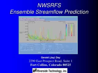
16. Temporal CorrelationBetween Forecasts and Analysis Corr., GEFS Control Fcst Nehalem River, FOSS OR A Small Basin in the West High Corr. for all lead times 0.5 Potomac River, Washington DC Corr. close to 1 for 1-2 day lead, Decreasing to 0 at day 10 Corr., GEFS Ens. Mean Fcst ----- GEFS members ----- Mean of GEFS mem. ----- GEFS control ----- GFS high resolution ----- GEFS Ens. Mean 0.0

17. Correlation Coefficient as Function of Lead Time and Mean FlowThe high resolution GFS forecast has lower correlation, especially for day 2-5 over small basins and for week 2 forecast over largest basins. Major Improvement due to ensemble approach. Ranges m**3/s >2000 1000-2000 500-1000 300-500 200-300 150-200 120-150 90-120 70-90 55-70 45-55 40-45 35-40 30-35 25-30 20-25 15-20 10-15 1-10 0-1 GFS-CTL Difference CTL Ranges m**3/s >2000 1000-2000 500-1000 300-500 200-300 150-200 120-150 90-120 70-90 55-70 45-55 40-45 35-40 30-35 25-30 20-25 15-20 10-15 1-10 0-1 ENSEMBLE Mean -CTL Difference Mean Score of GEFS Members -CTL Difference

18. CRPSS • Continuous Ranked Probability Score (CRPS) • The integral of the Brier scores at all possible threshold values for a continuous predictand (Hersbach 2000; Toth et al. 2003) • Averaged over the test data • Reduces to Mean Absolute Error (MAE) for a single value (deterministic) forecast. • CRPS is calculated for • GFS high resolution (single) forecast • GEFS control (single) forecast • GEFS 10-member mean (deterministic-style) forecast • Probabilistic forecast based on GEFS 10 member ensemble • Continuous Ranked Probability Skill Score CRPSS=1-CRPS/CRPS_ref • Reference forecast: persistent forecast (forecast=initial) • Not the best choice. Generating forecast without precip. Forcing is an alternative • CRPSS is less or equal to 1.0 • <=0, no skill compared with reference forecast • >0, some skill over the reference forecast

19. CRPSS of Various Forecasts (lead time 120h) CRPSS, GFS high res. CRPSS, GEFS Control CRPSS Ens. Mean Fcst CRPSS, Ensemble

20. CRPSS as a Function of Lead Time and Mean Flow, Raw ForecastsSlight Improvement due to ensemble approachMajor Improvement due to probabilistic forecastHigh resolution GFS is superior for 2-8 day lead Ranges m**3/s >2000 1000-2000 500-1000 300-500 200-300 150-200 120-150 90-120 70-90 55-70 45-55 40-45 35-40 30-35 25-30 20-25 15-20 10-15 1-10 0-1 GFS-CTL Difference CTL Ranges m**3/s >2000 1000-2000 500-1000 300-500 200-300 150-200 120-150 90-120 70-90 55-70 45-55 40-45 35-40 30-35 25-30 20-25 15-20 10-15 1-10 0-1 ENSEMBLE MEAN -CTL Difference ENSEMBLE PROBABILISTIC -CTL Difference

21. + - CDF + Mean of Forecast Analysis |Fmean-A|>0 Spread>0 CDF CDF |Fmean-A|=0 Spread>0 Mean of Forecast Analysis Mean of Forecast =Analysis In the situation where 1st moment error exists (|Fmean-A|>0), CRPS is minimized if Spread ~ |Fmean-A| (an idealized ensemble). How CRPS Reflects Errors in 1st (position) and 2nd (dispersion) Moments? |F-A|>0 Spread=0 CRPS Decreases With Increased spread CDF CRPS is smaller if (1) the analysis is closer to the mean of the forecast pdf and (2) spread is smaller (CRPS=0 for a perfect deterministic forecast). Forecast Analysis CRPS can be reduced by bias correction (adjustment of the first moment) and/or spread inflation (adjustment of the second moment)

22. CRPSS as Function of Lead Time and Mean Flow, After Bias-reduction (Using dependent training data set, not a practical bias correction)Slight/major Improvement due to ensemble approach/probabilistic forecastHigh resolution GFS is not as good as the ensemble control Ranges m**3/s >2000 1000-2000 500-1000 300-500 200-300 150-200 120-150 90-120 70-90 55-70 45-55 40-45 35-40 30-35 25-30 20-25 15-20 10-15 1-10 0-1 GFS-CTL Difference CTL Ranges m**3/s >2000 1000-2000 500-1000 300-500 200-300 150-200 120-150 90-120 70-90 55-70 45-55 40-45 35-40 30-35 25-30 20-25 15-20 10-15 1-10 0-1 ENSEMBLE MEAN -CTL Difference ENSEMBLE PROBABILISTIC -CTL Difference

23. CRPSS as a Function of Lead Time and Mean Flow, Raw Forecasts Slight Improvement due to ensemble approachMajor Improvement due to probabilistic forecastHigh resolution GFS is superior for 2-8 day lead Ranges m**3/s >2000 1000-2000 500-1000 300-500 200-300 150-200 120-150 90-120 70-90 55-70 45-55 40-45 35-40 30-35 25-30 20-25 15-20 10-15 1-10 0-1 GFS-CTL Difference CTL Ranges m**3/s >2000 1000-2000 500-1000 300-500 200-300 150-200 120-150 90-120 70-90 55-70 45-55 40-45 35-40 30-35 25-30 20-25 15-20 10-15 1-10 0-1 ENSEMBLE MEAN -CTL Difference ENSEMBLE PROBABILISTIC -CTL Difference

24. Effect of Bias CorrectionCRPSS of The Ensemble Based Probabilistic Forecast(Averaged over selected ranges of mean Stream Flow) After Bias-reduction Without Bias-reduction >2000m**3/s 1000-2000 >2000m**3/s 1000-2000 500-1000 300-500 500-1000 300-500 0 0 • Observations: • Positive skill for the large river basins in raw forecast. • Improvement due to bias-correction. • Positive skill for (almost) all river basins after bias correction • lower skill for 3-7 day lead, small and medium basins. 200-300 70-90 35-45 15-20 Ranges: (m**3/s) >2000m 1000-2000 500-1000 300-500 200-300 70-90 35-45 15-20 200-300 70-90 35-45 15-20 Discussion: Operationally practical bia-correction algorithms may have similar (although less striking) effect.

25. CRPSS • Lack of skill for small and medium basins with 3-7 days lead, even after bias correction • Possible explanation: • Bias and insufficient spread in the streamflow forecast • due to deficiencies in the forcing (precipitation and/or runoff forecast) generated by the GEFS system • Bias • Insufficient spread on grid and subgrid scales. • Spatial and temporal resolution • Possible Solutions: • Downscaling of precipitation/runoff; • Bias correction of precipitation/runoff. ----- GEFS members ----- GEFS ens. mean ----- GEFS control ----- GFS high resolution ----- NLDAS Single Case Ensemble April 1st, 2006 Average over 60 cases Ordered Ensemble May 4th

26. Conclusions and Discussions • Distributed river routing system (coupled GEFS, NOAH and the Lohmann River Flow model) generates reasonable gridded river flow forecast. • The coupled GFS-Noah system provides reasonable forcing to the river routing model • The ensemble approach, especially the ensemble-based probabilistic forecast, improves the forecast skill significantly. • Ensemble spread is comparable to the forecast error in first moment • Large basin forecasts are more skillful with higher correlation and positive CRPSS for all lead times up to 16 days. • GEFS provides reasonable forcing • Medium/small basin forecasts, especially for short to medium lead time, suffer from underdispersion (insufficient spread). • Downscaling of hydro-meteorological forcing is needed. • Forecast can be improved and calibrated through bias correction. • For the small and medium basins at lead time of 2-7 days, the high resolution GFS forecast is superior to the lower resolution runs in that it has smaller bias, but this is balanced by lower forecast-analysis correlation. • The GEFS ensemble, with suitable post processing, can outperform higher resolution single forecast

27. Evaluation Using actual USGS streamflow observations at unregulated basins. (Ohio River, in corporation with Ohio RFC) Corporation initiatives from other RFCs welcome Configuration Expand to global domain (at 0.5 degree resolution) Improvement of the Forcing (precipitation/runoff) Bias correction Downscaling Calibration of the Product (post-processing of streamflow forecast) Bias correction to the streamflow output for better product. Generate a hind-cast data set for a better estimate of bias. Further Development Plan

28. Thank You!

29. Background

30. RMS Error Before After Before After Absolute bias error QUALITATIVE COMPARISON OF ADAPTIVE BIAS CORRECTION & DOWNSCALING METHODS WITH EXISTING APPROACHES Dave Rudack Stensrud and Yussouf 2005 FIG. 5. Values of root-mean-square error (K) plotted as a function of forecast hour for (top) 2-m temperature from the full 31 member BCE (blue), the NCEP-only BCE (red), and the AVN (solid black line) and Eta (dashed line) MOS. Results are calculated at 1258 station locations for both the ensemble and AVN and Eta MOS data (after Stensrud and Yussouf 2005).

31. REAL-TIME GENERATION OF HIND-CAST DATASET? Today’s Julian Date TJD TJD + 30 TJD - 30 Actual ensemble generated today 2006 Time 2005 2004 2003 1968 1967 Hind-casts for TJD+30 generated today Hind-casts (or its statistics) for TJD+/- 30 saved on disc

32. Forecast Example (initiated April 1st, 2006) Stream Flow Forced by GFS,GEFS Forecast and NLDAS ProductForecast Starting at 00Z, April 1st, 2006. Lead time 15 days GFS High Res. Ensemble (low res.) Control Single control forecasts similar to each other; Ensemble mean is similar to the analysis. This suggests the ensemble mean has its value in stream flow forecast. Ensemble Mean Analysis (NLDAS)

33. Forecast Example (initiated April 1st, 2006) Stream Flow Stream Flow, Analysis and Ensemble Mean ForecastAbsolute Error of Ensemble Mean and Ensemble SpreadForecast Starting at 00Z, April 1st, 2006. lead time 12 days Analysis (NLDAS) Ensemble Mean Same as previous slide except for the error, where absolute value is plotted to compared with the spread. Spread is comparable to error, but the value is smaller, especially in the West. Absolute Error Ensemble Spread

34. Nehalem River, FOSS OR A Small Basin A challenge for the models. April 1st, large forecast discrepancy from day 1 despite significant spread • Possible causes of the problem in the short range forecast • Lack of spread in precip. fcst. on grid and subgrid scale. • Spatial and temporal resolution of the runoff. • Bias of precipitation (and runoff) forecast ----- GEFS members ----- GEFS ens. mean ----- GEFS control ----- GFS high resolution ----- NLDAS April 1st 0 2 4 6 8 10 12 14 16 Lead Time (days) May 4th

35. Merrimack-Concord River Lowell, MA A Medium Sized Basin Major Problem Underdispersive ensemble in grid and subgrid scale precipitation. Mid-May Flood Event Compared with the Early-April event, the Mid-May event is harder for the model to simulate. Nevertheless, the ensemble shows some skill indicating a major event with 10+ day lead, various amplitude and timing. Early April Major event forecast despite short range over- forecast ----- GEFS members ----- GEFS ens. mean ----- GEFS control ----- GFS high resolution ----- NLDAS May 4th 0 2 4 6 8 10 12 14 16 Lead Time (days) 0 2 4 6 8 10 12 14 16 Lead Time (days) April 1st

36. CRPSS of Various Forecasts (lead time 360h)(After Bias-correction with dependenttraining period) CRPSS, GFS high res. CRPSS, GFS low res. CRPSS Ens. Mean Fcst CRPSS, Ensemble

37. --- GFS --- CTL --- ENS. MEAN --- ENSEMBLE Category-mean of CRPSS (Probabilistic based on GEFS)Slight Improvement due to ensemble approachMajor Improvement due to probabilistic forecastHigh res. GFS is superior for 2-8 day lead, small and medium basins Category 19, 1000-2000m**3/s Category 15, 150-200m**3/s Category 11, 55-70m**3/s Category 07, 30-35m**3/s

38. Effect of Bias CorrectionCRPSS of Ensemble Control and Ensemble(Lead Time 240h; before and after bias-correction) Ens. control, Before Ens. Control, After Ensemble, Before Ensemble, After

39. --- GFS --- CTL --- ENS. MEAN --- ENSEMBLE Category-mean of CRPSS, After Bias Correction (Probabilistic Forecast based on GEFS)High res. GFS is NOT superior Category 19, 1000-2000m**3/s Category 15, 150-200m**3/s Category 07, 30-35m**3/s Category 11, 55-70m**3/s

40. Bias Correction withIndependent Training Data Set(Training: April; Evaluation: May) CTL, Before CTL, After ENSEMBLE, After ENSEMBLE, Before