Download
1 / 24
240 likes | 597 Views
Estimation Procedures. Introduction. Interval estimates Consists of a range of values (an interval) instead of a point E.g., an interval estimate is usually phrased as “ from 39% to 45% of the electorate will vote for the candidate

E N D
Introduction • Interval estimates • Consists of a range of values (an interval) instead of a point • E.g., an interval estimate is usually phrased as “from 39% to 45% of the electorate will vote for the candidate • May also be phrased as 42% plus or minus 3 percentage points of the population will vote for the candidate (the same as between 39% and 45%)
Unbiased Estimators • Samplestatistics are used as the estimators of populationparameters • Two sample statistics are unbiased estimators and so are the best ones to use: • Means • Proportions • An estimator is unbiased if and only if the mean of its sampling distribution is equal to the population value of interest • Sample means conform to this criterion
Sample Proportions as Unbiased Estimators • Sample proportions (P sub s) are unbiased estimators of population proportions • If we do a sampling distribution of the proportions in many samples, the sampling distribution of sample proportions will have a mean (µp) equal to the population proportion (Pu) • All other sample statistics are biased
Efficiency • A good estimator must be relatively efficient • The more efficient the estimate, the more the sampling distribution is clustered around the mean • This is a matter of dispersion, so we will be talking about the standard deviation of the sampling distribution (also called the standarderrorof the mean) • With larger samples (e.g., N=16), the population distribution will be 4 times larger than the sampling distribution
Efficiency • As sample size increases, the standard deviation of the sample means will decrease, making it a more efficient estimator • We know that because as the denominator increases, the number will decrease in size • E.g., ½, ¼, 1/8, 1/10, 1/15 • The efficiency of any estimator can be improved by increasing the sample size
Procedure for Constructing an Interval Estimate • First step in constructing an interval estimate • Decide on the risk you are willing to take of being wrong (which is the confidence level) • An interval estimate is wrong if it does not include the population value • The probability that an interval estimate does not include the population value is called alpha • An alpha level of 0.05 is the same as a confidence level of 95% • The most commonly used confidence level is 95%
Second Step • Picture the sampling distribution and divide the probability of error equally into the upper and lower tails of the distribution and find the corresponding Z score • If we set alpha equal to 0.05 (95% confidence level), we would place half (-.025) of this probability in the lower tail and half in the upper tail of the distribution • We need to find the Z score beyond which lies a proportion of .0250 of the total area • To do this, go down Column C of Appendix A until you find this proportion (.0250) • The associated Z score is 1.96
Since we are interested in both the upper and lower tails, we designate the Z score that corresponds to an alpha of .05 as plus or minus 1.96 • So, we are looking for a Z score that encloses 95% of the normal curve
Other Confidence Levels • Besides the 95% level, there are two other commonly used confidence levels • First is 90% level (alpha = .10) • Where we have a 10 percent chance of making a mistake • Will have a Z score of plus or minus 1.65 • Second is 99% level (alpha = .01) • We have a 1 % chance of making a mistake • Will have a Z score of plus or minus 2.58
Interval Estimation Procedures for Sample Means (confidence intervals) • After deciding on a confidence level, you can construct a confidence interval • Formula 7.1 for the confidence interval
Estimating the Standard Deviation of the Population • In the I.Q. example, we knew the population standard deviation of IQ scores • But for most all variables, we won’t know the population standard deviation • We do know what the standard deviation of our sample is, since we can calculate it after we finish our study • We can estimate the population standard deviation with the standard deviation of the sample • But s is a biased estimator, so the formula needs to be changed slightly to correct for the bias • For larger samples the bias of s will not affect the interval very much
The revised formula for cases in which the population standard deviation is unknown:
The substitution of the sample standard deviation for the population standard deviation is permitted only for large samples (samples with 100 or more cases) • You have to now divide by N-1, because we did not do that when calculating the standard deviation of the sample • You can construct interval estimates for samples smaller than 100, but need to use the Student’s t distribution (Appendix B) which will be covered in Chapter 8, instead of the Z distribution)
Formula for a Confidence Interval • The formula for a confidence interval is made up of two things: • The confidence level (Z) , and the size of a single standard deviation • Larger Z values result in wider confidence intervals (larger Z values = larger confidence levels) • Larger N values result in narrower confidence intervals
Interval Estimation Procedures for Sample Proportions (Large Samples) • Estimation procedures for sample proportions are about the same as those for sample means, but using a different statistic • We know from the Central Limit Theorem, that sample proportions have sampling distributions that are normal in shape
Sample Proportions • With the mean of the sampling distribution equal to the populationproportion • In addition, the standard deviation of the sampling distribution of sample proportions is equal to the following:
Estimating the Proportion in the Population • The dilemma is resolved by setting the value of P sub u at 0.5 • What this means is that the guess at the percentage of the population that agrees will be 50%, which is the most heterogeneous possibility • If set P sub u at .4, we are saying that 40% agree and 60% disagree, and the values of the expression will be .24, or less than if we guessed the percentage as 50% • So, 1 – P sub u will also be .5, and the entire expression will always have a value of 0.5 x 0.5 = .25 • This is the maximum value this expression can attain • The interval will be at a maximum width—this is the most conservative solution possible
Controlling the Width of Interval Estimates • The width of an interval estimate for either sample means or sample proportions can be partly controlled by manipulating two terms in the equation • The confidence level can be raised or lowered • The exact confidence level (or alpha level) will depend, in part, on the purpose of the research
Confidence Level Choices • If dealing with harmful effects of drugs, you would demand very high levels of confidence (99.9%) • If the intervals are only for guesstimates, then lower confidence levels can be used (such as 90%) • The intervals widen as confidence levels increase (you want the intervals to be narrow) • When you move from 90% confidence level to 95% to 99%, the intervals will get wider • So may have an interval of 10 percentage points, which is most often too large to make a prediction • May have to say that 45% of the population will vote for a candidate, plus or minus 10% (between 35% and 55% will vote for a candidate)
Changing Interval Widths • Second, the interval width can be increased or decreased by gathering samples of different sizes • Sample size bears the opposite relationship to interval width • As sample size increases, confidence interval width decreases • The decrease in interval width does not bear a linear relationship with sample size • N might have to be increased four times to double the accuracy • Therefore, there are diminishing returns with increases in the sample size
Estimating Sample Size • If you want a particular confidence interval, of say plus or minus 3%, can decide, before you do the study, about how large the sample needs to be