Download
1 / 25
250 likes | 409 Views
Detailed evolution of performance metrics. Folding. Judit Gimenez (judit@bsc.es ). Petascale workshop 2013. Our Tools. Since 1991 Based on traces Open Source http://www.bsc.es/paraver Core tools: Paraver ( paramedir ) – offline trace analysis Dimemas – message passing simulator

E N D
Detailed evolution of performance metrics Folding Judit Gimenez (judit@bsc.es) Petascaleworkshop 2013
Our Tools • Since 1991 • Based on traces • Open Source • http://www.bsc.es/paraver • Core tools: • Paraver (paramedir) – offline trace analysis • Dimemas – message passing simulator • Extrae – instrumentation • Performance analytics • Detail, flexibility, intelligence • Behaviour vs syntactic structure
What is a good performance? • Performance of a sequential region = 2000 MIPS Isitgoodenough? Isiteasytoimprove?
What is a good performance? MR. GENESIS Interchanging loops
Can I get very detailed perf. data with low overhead? • Application granularity vs. detailed granularity • Samples: hardware counters + callstack • Folding:based on known structure: iterations, routines, clusters; • Project all samples into one instance • Extremely detailed time evolution of hardware counts, rates and callstack with minimal overhead • Correlate many counters • Instantaneous CPI stack models UnveilingInternalEvolution of ParallelApplicationComputationPhases (ICPP 2011)
Mixing instrumentation and sampling • Benefit from applications’ repetitiveness • Different roles • Instrumentation delimits regions • Sampling reports progress within a region Synthetic Iteration Iteration #1 Iteration #2 Iteration #3 UnveilingInternalEvolution of ParallelApplicationComputationPhases (ICPP 2011)
Folding hardware counters • Instructions evolution for routine copy_faces of NAS MPI BT.B • Red crosses represent the folded samples and show the completed instructions from the start of the routine • Green line is the curve fitting of the folded samples and is used to reintroduce the values into the tracefile • Blue line is the derivative of the curve fitting over time (counter rate)
Folding hardware counters with call stack Folded source code line Folded instructions
Using Clustering to identify structure Bursts Duration Automatic Detection of Parallel Applications Computation Phases. (IPDPS 2009)
Example 1: PEPC do i = 1, n htable(i)%node = 0 htable(i)%key = 0 htable(i)%link = -1 htable(i)%leaves = 0 htable(i)%childcode = 0 End do htable%node = 0 htable%key = 0 htable%link = -1 htable%leaves = 0 htable%childcode = 0 A 96 MIPS
Example 1: PEPC A B 403 MIPS
Example 2: CG-POP with CPI-Stack iter_loop: do m = 1, solv_max_iters sumN1=c0 sumN3=c0 do i=1,nActive Z(i) = Minv2(i)*R(i) sumN1 = sumN1 + R(i)*Z(i) sumN3 = sumN3 + R(i)*R(i) enddo do i=iptrHalo,n Z(i) = Minv2(i)*R(i) enddo call matvec(n,A,AZ,Z) sumN2=c0 do i=1,nActive sumN2 = sumN2 + AZ(i)*Z(i) enddo call update_halo(AZ) ... do i=1,n stmp = Z(i) + cg_beta*S(i) qtmp = AZ(i) + cg_beta*Q(i) X(i) = X(i) + cg_alpha*stmp R(i) = R(i) - cg_alpha*qtmp S(i) = stmp Q(i) = qtmp enddo end do iter_loop B A B C D C D Framework for a Productive Performance Optimization (PARCO Journal 2013) • Folded lines • Interpolation statistic profile • Points to “small” regions A pcg_chrongear_linear matvec Line number
Example 2: CG-POP sumN1=c0 sumN3=c0 do i=1,nActive Z(i) = Minv2(i)*R(i) sumN1 = sumN1 + R(i)*Z(i) sumN3 = sumN3 + R(i)*R(i) enddo do i=iptrHalo,n Z(i) = Minv2(i)*R(i) enddo iter_loop: do m = 1, solv_max_iters sumN2=c0 call matvec_r(n,A,AZ,Z,nActive,sumN2) call update_halo(AZ) ... sumN1=c0 sumN3=c0 do i=1,n stmp = Z(i) + cg_beta*S(i) qtmp = AZ(i) + cg_beta*Q(i) X(i) = X(i) + cg_alpha*stmp R(i) = R(i) - cg_alpha*qtmp S(i) = stmp Q(i) = qtmp Z(i) = Minv2(i)*R(i)} if (i <= nActive) then} sumN1 = sumN1 + R(i)*Z(i) sumN3 = sumN3 + R(i)*R(i) endif enddo end do iter_loop iter_loop: do m = 1, solv_max_iters sumN1=c0 sumN3=c0 do i=1,nActive Z(i) = Minv2(i)*R(i) sumN1 = sumN1 + R(i)*Z(i) sumN3 = sumN3 + R(i)*R(i) enddo do i=iptrHalo,n Z(i) = Minv2(i)*R(i) enddo call matvec(n,A,AZ,Z) sumN2=c0 do i=1,nActive sumN2 = sumN2 + AZ(i)*Z(i) enddo call update_halo(AZ) ... do i=1,n stmp = Z(i) + cg_beta*S(i) qtmp = AZ(i) + cg_beta*Q(i) X(i) = X(i) + cg_alpha*stmp R(i) = R(i) - cg_alpha*qtmp S(i) = stmp Q(i) = qtmp enddo end do iter_loop B CD C D AB A
Example 2: CG-POP • 11% improvement on an already optimized code B C A D CD AB CD AB
Example 3: CESM 4 cycles in Cluster 1 • Group A: • conden: 2.7% • compute_uwshcu: 3.3% • rtrnmc: 1.75% • Group B: • micro_mg_tend: 1.36% (1.73%) • wetdepa_v2: 2.5% • Group C: • reftra_sw: 1.71% • spcvmc_sw: 1.21% • vrtqdr_sw 1.43% A B C
Example 3: CESM • Consists of a double nested loop • Very long ~400 lines • Unnecessary branches with inhibit vectorization • Restructuring wetdepa_v2 • Break up long loop to simplify vectorization • Promote scalar to vector temporaries • Common expression elimination
Energy counters @ SandyBridge • 3 Energy Domains • Processor die (Package) • Cores (PP0) • Attached RAM (optional, DRAM) • In comparison with performance counters • Per processor die information • Time discretization • Measured at 1Khz No control on boundaries (f.i separate MPI from computing) • Power quantization • Energy reported in multiples of 15.3 µJoules • Folding energy counters • Noise values • Discretization – consider a uniform distribution? • Quantization – select the latest valid measure?
Folding energy counters in serial benchmarks MIPSCoreDRAMPACKAGETDP FT.B LU.B Stream BT.B 435.gromacs 437.leslie3d 444.namd 481.wrf
HydroC analysis 1 pps 2pps 4 pps 8pps • HydroC, 8 MPI processes • Intel® Xeon® E5-2670 @ 2.60GHz (2 x octo-core nodes)
MrGenesis analysis 1 pps 2pps 4 pps 8pps • MrGenesis, 8 MPI processes • Intel® Xeon® E5-2670 @ 2.60GHz (2 x octo-core nodes)
Performance answers are in detailed and precise analysis Analysis: [temporal] behaviourvs syntactic structure www.bsc.es/paraver Conclusions