Download
1 / 37
370 likes | 514 Views
MOD06 Cloud Top Properties. Richard Frey Paul Menzel Bryan Baum University of Wisconsin - Madison. CTPs using CO2 Slicing. Different ratios reveal cloud properties at different levels hi - 14.2/13.9 mid - 13.9/13.6 low - 13.6/13.3 Meas Calc p c

E N D
MOD06 Cloud Top Properties Richard Frey Paul Menzel Bryan Baum University of Wisconsin - Madison
CTPs using CO2 Slicing • Different ratios reveal cloud properties • at different levels • hi - 14.2/13.9 • mid - 13.9/13.6 • low - 13.6/13.3 • Meas Calc • pc • (I1-I1clr) 11 dB1 • ps • ----------- = ---------------- • pc • (I2-I2clr) 22 dB2 • ps • if (Iclr- I) < Δ • then IRW is used
MODIS Algorithm Improvements before Collect 6 Collect 3. night-time cloud phase introduced Collect 4. destriping started, instrument IR calibration improved Collect 5. cloud mask improved (deserts, poles, night), radiance bias adjustment for measured versus calculated introduced
MODIS Algorithm Adjustments for Collect 6 A: Implement Band 34, 35, 36 spectral shifts suggested by Tobin et al. (2005) for Aqua. B: Use "top-down” channel pairs 36/35, 35/34, 34/33 in that order to select CTP. C: Lower "noise" thresholds (clear minus cloudy radiances required to indicate cloud presence in bands 33 to 36) to force more CO2 slicing solutions for high thin clouds. D: Restrict CO2 channel pair solutions to appropriate portion of troposphere (determined by weighting functions – 36/35 < 450 hPa, 35/34 < 550 hPa, and 34/33 < 650 hPa). E: Adjust ozone profile between 10 and 100 hPa to GDAS values instead of using climatology (so that CO2 radiances influenced by O3 profiles are calculated correctly). F: Use CO2 = [mx+a*sin(2πx/365)]+b where m = 1.5 ppmv / 365, b = 337.5 ppmv, a = 3 ppmv, and x = # days since 1 Jan 1980 to accommodate CO2 increase. G: Prohibit CO2 slicing solutions for water clouds; use only IRW solution. Avoid IRW solutions for ice clouds; use CO2 slicing whenever possible. H: Add marine stratus improvement where a constant lapse rate is assumed in low level inversions – lapse rate is adjusted according to latitude region. I. Add stratospheric cloud flag responding to BT13.9>BT13.3+0.5.
MODIS Algorithm Adjustments for Collect 6 A: Implement Band 34, 35, 36 spectral shifts suggested by Tobin et al. (2005) for Aqua. B: Use "top-down” channel pairs 36/35, 35/34, 34/33 in that order to select CTP. C: Lower "noise" thresholds (clear minus cloudy radiances required to indicate cloud presence in bands 33 to 36) to force more CO2 slicing solutions for high thin clouds. D: Restrict CO2 channel pair solutions to appropriate portion of troposphere (determined by weighting functions – 36/35 < 450 hPa, 35/34 < 550 hPa, and 34/33 < 650 hPa). E: Adjust ozone profile between 10 and 100 hPa to GDAS values instead of using climatology (so that CO2 radiances influenced by O3 profiles are calculated correctly). F: Use CO2 = [mx+a*sin(2πx/365)]+b where m = 1.5 ppmv / 365, b = 337.5 ppmv, a = 3 ppmv, and x = # days since 1 Jan 1980 to accommodate CO2 increase. G: Prohibit CO2 slicing solutions for water clouds; use only IRW solution. Avoid IRW solutions for ice clouds; use CO2 slicing whenever possible. H: Add marine stratus improvement where a constant lapse rate is assumed in low level inversions – lapse rate is adjusted according to latitude region. I. Add stratospheric cloud flag responding to BT13.9>BT13.3+0.5.
MODIS Algorithm Adjustments for Collect 6 A: Implement Band 34, 35, 36 spectral shifts suggested by Tobin et al. (2005) for Aqua. B: Use "top-down” channel pairs 36/35, 35/34, 34/33 in that order to select CTP. C: Lower "noise" thresholds (clear minus cloudy radiances required to indicate cloud presence in bands 33 to 36) to force more CO2 slicing solutions for high thin clouds. D: Restrict CO2 channel pair solutions to appropriate portion of troposphere (determined by weighting functions – 36/35 < 450 hPa, 35/34 < 550 hPa, and 34/33 < 650 hPa). E: Adjust ozone profile between 10 and 100 hPa to GDAS values instead of using climatology (so that CO2 radiances influenced by O3 profiles are calculated correctly). F: Use CO2 = [mx+a*sin(2πx/365)]+b where m = 1.5 ppmv / 365, b = 337.5 ppmv, a = 3 ppmv, and x = # days since 1 Jan 1980 to accommodate CO2 increase. G: Prohibit CO2 slicing solutions for water clouds; use only IRW solution. Avoid IRW solutions for ice clouds; use CO2 slicing whenever possible. H: Add marine stratus improvement where a constant lapse rate is assumed in low level inversions – lapse rate is adjusted according to latitude region. I. Add stratospheric cloud flag responding to BT13.9>BT13.3+0.5.
MODIS C6: CO2 changes over time Mauna Loa Parameterization
MODIS Algorithm Adjustments for Collect 6 A: Implement Band 34, 35, 36 spectral shifts suggested by Tobin et al. (2005) for Aqua. B: Use "top-down” channel pairs 36/35, 35/34, 34/33 in that order to select CTP. C: Lower "noise" thresholds (clear minus cloudy radiances required to indicate cloud presence in bands 33 to 36) to force more CO2 slicing solutions for high thin clouds. D: Restrict CO2 channel pair solutions to appropriate portion of troposphere (determined by weighting functions – 36/35 < 450 hPa, 35/34 < 550 hPa, and 34/33 < 650 hPa). E: Adjust ozone profile between 10 and 100 hPa to GDAS values instead of using climatology (so that CO2 radiances influenced by O3 profiles are calculated correctly). F: Use CO2 = [mx+a*sin(2πx/365)]+b where m = 1.5 ppmv / 365, b = 337.5 ppmv, a = 3 ppmv, and x = # days since 1 Jan 1980 to accommodate CO2 increase. G: Prohibit CO2 slicing solutions for water clouds; use only IRW solution. Avoid IRW solutions for ice clouds; use CO2 slicing whenever possible. H: Add marine stratus improvement where a constant lapse rate is assumed in low level inversions – lapse rate is adjusted according to latitude region. I. Add stratospheric cloud flag responding to BT13.9>BT13.3+0.5.
Avoid IRW solutions for ice clouds Number for Aug 2006 1 CTH MODIS - CALIOP IRW CTHs are too low for ice clouds
Avoid CO2 slicing solutions for water clouds Number for Aug 2006 CTH MODIS - CALIOP Number for Aug 2006 CTH MODIS - CALIOP
Determine C6 Cloud Phase with Beta Ratio Tests • Collection 5: • Based on 8.5/11-µm brightness temperatures (BT) and their differences (BTD) • Collection 6: • Supplement BT & BTD tests with emissivity ratios (b ratio) • b ratios are based on 7.3, 8.5, 11, 12-µm bands (more on another slide) 8.5/11: has the most sensitivity to cloud phase 11/12: sensitive to cloud opacity; implementation of this pair helps with optically thin clouds (improves phase discrimination for thin cirrus) 7.3/11: sensitive to high versus low clouds; helps with low clouds (one of the issues was a tendency for low-level water clouds to be ringed with ice clouds as the cloud thinned out near the edges) • Use of b ratio mitigates influence of the surface • Approach imposes new requirements: • - clear-sky radiances, which implies knowledge of… • - atmospheric profiles, surface emissivity, and a fast RT model
The Beta ratio is based on cloud emissivity profiles A cloud emissivity profile for a single band: e(p) = (I-Iclr) ––––––––––––––––––––––––––– [Iac(p) + Tac(p)Ibb(p) – Iclr)] where Iclr = clear-sky radiance Iac(p) = above cloud emission at pressure p Ibb(p) = TOA radiance for opaque cloud at pressure p Tac(p)= above cloud transmission bx,y(p) = ln[1-ec,y(p)] –––––––––––––– ln[1-ec,x(p)] where x and y are two channels used to compute the ratio
MODIS IR Phase for a granule on 28 August, 2006 at 1630 UTC Over N. Atlantic Ocean between Newfoundland and Greenland False color image Red: 0.65 mm; Green: 2.1 mm; Blue: 11 mm Thin cirrus: blue Opaque ice clouds: pink Water clouds: white/yellow Snow/ice: magenta (Southern tip of Greenland) Ocean: dark blue Land: green Collection 5 algorithm but with uncertain and mixed phase pixels combined into “uncertain” category
MODIS IR Phase for a granule on 28 August, 2006 at 1630 UTC Over N. Atlantic Ocean between Newfoundland and Greenland False color image Red: 0.65 mm; Green: 2.1 mm; Blue: 11 mm Collection 6 algorithm: Propose 3 categories, deleting mixed phase since there is no justification for this category
For C5, most of the uncertain phase pixels occurred in the storm tracks, i.e., at high latitudes For C6, there are many less uncertain phase retrievals now that cirrus is more likely to be identified as ice phase clouds
MODIS Algorithm Adjustments for Collect 6 A: Implement Band 34, 35, 36 spectral shifts suggested by Tobin et al. (2005) for Aqua. B: Use "top-down” channel pairs 36/35, 35/34, 34/33 in that order to select CTP. C: Lower "noise" thresholds (clear minus cloudy radiances required to indicate cloud presence in bands 33 to 36) to force more CO2 slicing solutions for high thin clouds. D: Restrict CO2 channel pair solutions to appropriate portion of troposphere (determined by weighting functions – 36/35 < 450 hPa, 35/34 < 550 hPa, and 34/33 < 650 hPa). E: Adjust ozone profile between 10 and 100 hPa to GDAS values instead of using climatology (so that CO2 radiances influenced by O3 profiles are calculated correctly). F: Use CO2 = [mx+a*sin(2πx/365)]+b where m = 1.5 ppmv / 365, b = 337.5 ppmv, a = 3 ppmv, and x = # days since 1 Jan 1980 to accommodate CO2 increase. G: Prohibit CO2 slicing solutions for water clouds; use only IRW solution. Avoid IRW solutions for ice clouds; use CO2 slicing whenever possible. H: Add marine stratus improvement where a constant lapse rate is assumed in low level inversions – lapse rate is adjusted according to latitude region. I. Add stratospheric cloud flag responding to BT13.9>BT13.3+0.5.
Marine Stratus CTH Over-Estimated MODIS CTH CALIOP CTH
Marine Stratus Correction for Low Level Inversion Modified (Minnis 1992) Current 31
The apparent lapse rates are based on 11-micron differences between clear-sky and measured cloud radiances. Regression coefficients are based on latitude, using curve fitting for three different segments as shown above. Coefficients are provided for each month.
MODIS Algorithm Adjustments for Collect 6 A: Implement Band 34, 35, 36 spectral shifts suggested by Tobin et al. (2005) for Aqua. B: Use "top-down” channel pairs 36/35, 35/34, 34/33 in that order to select CTP. C: Lower "noise" thresholds (clear minus cloudy radiances required to indicate cloud presence in bands 33 to 36) to force more CO2 slicing solutions for high thin clouds. D: Restrict CO2 channel pair solutions to appropriate portion of troposphere (determined by weighting functions – 36/35 < 450 hPa, 35/34 < 550 hPa, and 34/33 < 650 hPa). E: Adjust ozone profile between 10 and 100 hPa to GDAS values instead of using climatology (so that CO2 radiances influenced by O3 profiles are calculated correctly). F: Use CO2 = [mx+a*sin(2πx/365)]+b where m = 1.5 ppmv / 365, b = 337.5 ppmv, a = 3 ppmv, and x = # days since 1 Jan 1980 to accommodate CO2 increase. G: Prohibit CO2 slicing solutions for water clouds; use only IRW solution. Avoid IRW solutions for ice clouds; use CO2 slicing whenever possible. H: Add marine stratus improvement where a constant lapse rate is assumed in low level inversions – lapse rate is adjusted according to latitude region. I. Add stratospheric cloud flag responding to BT13.9>BT13.3+0.5.
Stratospheric Cloud Test Stratospheric clouds are identified when a more opaque band is found to be warmer than a less opaque band indicating detection of a positive lapse rate above an opaque cloud; thus when BT13.9 > BT13.3 + 0.5 K a yellow flag is indicated in the image on the right.
MODIS Algorithm Adjustments for Collect 6 • A: Implement Band 34, 35, 36 spectral shifts suggested by Tobin et al. (2005) for Aqua. • B: Use "top-down” channel pairs 36/35, 35/34, 34/33 in that order to select CTP. • C: Lower "noise" thresholds (clear minus cloudy radiances required to indicate cloud presence in bands 33 to 36) to force more CO2 slicing solutions for high thin clouds. • D: Restrict CO2 channel pair solutions to appropriate portion of troposphere (determined by weighting functions – 36/35 < 450 hPa, 35/34 < 550 hPa, and • 34/33 < 650 hPa). • E: Adjust ozone profile between 10 and 100 hPa to GDAS values instead of using climatology (so that CO2 radiances influenced by O3 profiles are calculated correctly). • F: Use CO2 = [mx+a*sin(2πx/365)]+b where m = 1.5 ppmv / 365, b = 337.5 ppmv, • a = 3 ppmv, and x = # days since 1 Jan 1980 to accommodate CO2 increase. • G: Prohibit CO2 slicing solutions for water clouds; use only IRW solution. Avoid IRW solutions for ice clouds; use CO2 slicing whenever possible. • H: Add marine stratus improvement where a constant lapse rate is assumed in low level inversions – lapse rate is adjusted according to latitude region. • Add stratospheric cloud flag responding to BT13.9>BT13.3+0.5. • MODIS Collect 6 improvements over Collect 5 • measured by CALIOP for August 2006
(MODIS–CALIOP) for All Clouds; August 2006 Based on Collection 5 MODIS 5-km CTH and Version 3 CALIOP 5-km CTH 3 2 1 0 MODIS-CALIOP (km) -1 (MODIS–CALIOP) for All Clouds for August 2006 Based on Collection 6 MODIS 5-km CTH and Version 3 CALIOP 5-km CTH -2 -3 -4 -5 -6 -7
The largest cloud height differences results from not using CO2 slicing (>15 km) Reducing the cloud detection threshold produced more high thin cloud retrievals, but also produced erroneously high CO2 CTH retrievals for low water clouds in the southern Pacific CO2 slicing (IRW) heights should be avoided for water (ice) clouds A high bias in marine stratus was identified in the MODIS retrievals; CTH algorithm problems in inversions will be mitigated assuming a wet lapse rate Adjusting the spectral response of the CO2 bands reduced CTH errors Selecting the spectral radiance ratio using a top down criteria improved high cloud detection Making multiple passes through large data sets was necessary Using CALIOP as a reference was invaluable Collect 6 Cloud Products should be the ten year reference Conclusions on CTP Algorithm Adjustments
Remaining Actions (1) Spectral shifts have been implemented for Aqua MODIS. Are spectral shifts necessary for Terra MODIS? Intercomparisons with IASI are beginning to indicate answers. (2) Flag multi-layer cloud situations.