Download
1 / 123
1.24k likes | 1.4k Views
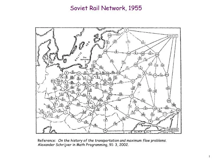
Soviet Rail Network, 1955. Reference: On the history of the transportation and maximum flow problems . Alexander Schrijver in Math Programming, 91: 3, 2002. Max flow and min cut. Two very rich algorithmic problems. Cornerstone problems in combinatorial optimization.

E N D
Soviet Rail Network, 1955 Reference: On the history of the transportation and maximum flow problems.Alexander Schrijver in Math Programming, 91: 3, 2002.
Max flow and min cut. Two very rich algorithmic problems. Cornerstone problems in combinatorial optimization. Beautiful mathematical duality. Nontrivial applications / reductions. Data mining. Open-pit mining. Project selection. Airline scheduling. Bipartite matching. Baseball elimination. Image segmentation. Network connectivity. Network reliability. Distributed computing. Egalitarian stable matching. Security of statistical data. Network intrusion detection. Multi-camera scene reconstruction. Many many more . . . Maximum Flow and Minimum Cut
Minimum Cut Problem • Flow network. • Abstraction for material flowing through the edges. • G = (V, E) = directed graph, no parallel edges. • Two distinguished nodes: s = source, t = sink. • c(e) = capacity of edge e. 2 5 9 10 15 15 10 4 source sink 5 s 3 6 t 8 10 15 4 6 10 15 capacity 4 7 30
Cuts • Def. An s-t cut is a partition (A, B) of V with s A and t B. • Def. The capacity of a cut (A, B) is: 2 5 9 10 15 15 10 4 5 s 3 6 t 8 10 A 15 4 6 10 15 Capacity = 10 + 5 + 15 = 30 4 7 30
Cuts • Def. An s-t cut is a partition (A, B) of V with s A and t B. • Def. The capacity of a cut (A, B) is: 2 5 9 10 15 15 10 4 5 s 3 6 t 8 10 A 15 4 6 10 15 Capacity = 9 + 15 + 8 + 30 = 62 4 7 30
Minimum Cut Problem • Min s-t cut problem. Find an s-t cut of minimum capacity. 2 5 9 10 15 15 10 4 5 s 3 6 t 8 10 15 4 6 10 A 15 Capacity = 10 + 8 + 10 = 28 4 7 30
2 5 9 10 15 15 10 4 5 s 3 6 t 8 10 15 4 6 10 15 4 7 30 Flows • Def. An s-t flow is a function that satisfies: • For each e E: (capacity) • For each v V – {s, t}: (conservation) • Def. The value of a flow f is: 0 4 0 0 0 4 0 4 4 0 0 0 0 capacity flow 0 0 Value = 4
2 5 9 10 15 15 10 4 5 s 3 6 t 8 10 15 4 6 10 15 4 7 30 Flows • Def. An s-t flow is a function that satisfies: • For each e E: (capacity) • For each v V – {s, t}: (conservation) • Def. The value of a flow f is: 6 10 6 0 0 4 3 8 8 1 10 0 0 capacity flow 11 11 Value = 24
2 5 9 10 15 15 10 4 5 s 3 6 t 8 10 15 4 6 10 15 4 7 30 Maximum Flow Problem • Max flow problem. Find s-t flow of maximum value. 9 10 9 1 0 0 4 9 8 4 10 0 0 capacity flow 14 14 Value = 28
Flows and Cuts • Flow value lemma. Let f be any flow, and let (A, B) be any s-t cut. Then, the net flow sent across the cut is equal to the amount leaving s. 6 2 5 9 10 6 0 10 15 15 0 10 4 4 3 8 8 5 s 3 6 t 8 10 A 1 10 15 0 0 4 6 10 15 11 11 Value = 24 4 7 30
Flows and Cuts • Flow value lemma. Let f be any flow, and let (A, B) be any s-t cut. Then, the net flow sent across the cut is equal to the amount leaving s. 6 2 5 9 10 6 0 10 15 15 0 10 4 4 3 8 8 5 s 3 6 t 8 10 A 1 10 15 0 0 4 6 10 15 11 Value = 6 + 0 + 8 - 1 + 11= 24 11 4 7 30
Flows and Cuts • Flow value lemma. Let f be any flow, and let (A, B) be any s-t cut. Then, the net flow sent across the cut is equal to the amount leaving s. 6 2 5 9 10 6 0 10 15 15 0 10 4 4 3 8 8 5 s 3 6 t 8 10 A 1 10 15 0 0 4 6 10 15 11 Value = 10 - 4 + 8 - 0 + 10= 24 11 4 7 30
Flows and Cuts • Flow value lemma. Let f be any flow, and let (A, B) be any s-t cut. Then • Pf. by flow conservation, all termsexcept v = s are 0
Flows and Cuts • Weak duality. Let f be any flow, and let (A, B) be any s-t cut. Then the value of the flow is at most the capacity of the cut. Cut capacity = 30 Flow value 30 2 5 9 10 15 15 10 4 5 s 3 6 t 8 10 A 15 4 6 10 15 Capacity = 30 4 7 30
Flows and Cuts • Weak duality. Let f be any flow. Then, for any s-t cut (A, B) we havev(f) cap(A, B). • Pf. • ▪ A B 4 8 t s 7 6
Certificate of Optimality • Corollary. Let f be any flow, and let (A, B) be any cut.If v(f) = cap(A, B), then f is a max flow and (A, B) is a min cut. Value of flow = 28Cut capacity = 28 Flow value 28 9 2 5 9 10 9 1 10 15 15 0 10 0 4 4 9 8 5 s 3 6 t 8 10 4 10 15 0 A 0 4 6 10 15 14 14 4 7 30
Towards a Max Flow Algorithm • Greedy algorithm. • Start with f(e) = 0 for all edge e E. • Find an s-t path P where each edge has f(e) < c(e). • Augment flow along path P. • Repeat until you get stuck. 1 0 0 20 10 30 0 t s 10 20 Flow value = 0 0 0 2
Towards a Max Flow Algorithm • Greedy algorithm. • Start with f(e) = 0 for all edge e E. • Find an s-t path P where each edge has f(e) < c(e). • Augment flow along path P. • Repeat until you get stuck. 1 20 0 0 X 20 10 20 30 0 t X s 10 20 Flow value = 20 20 0 0 X 2
Towards a Max Flow Algorithm • Greedy algorithm. • Start with f(e) = 0 for all edge e E. • Find an s-t path P where each edge has f(e) < c(e). • Augment flow along path P. • Repeat until you get stuck. locally optimality global optimality 1 1 20 0 20 10 20 10 20 10 30 20 30 10 t t s s 10 20 10 20 0 20 10 20 2 2 greedy = 20 opt = 30
Residual Graph • Original edge: e = (u, v) E. • Flow f(e), capacity c(e). • Residual edge. • "Undo" flow sent. • e = (u, v) and eR = (v, u). • Residual capacity: • Residual graph: Gf = (V, Ef ). • Residual edges with positive residual capacity. • Ef = {e : f(e) < c(e)} {eR : c(e) > 0}. capacity u v 17 6 flow residual capacity u v 11 6 residual capacity
Ford-Fulkerson Algorithm 2 4 4 capacity G: 6 8 10 10 2 10 s 3 5 t 10 9
Ford-Fulkerson Algorithm 0 flow 2 4 4 capacity G: 0 0 0 6 0 8 10 10 2 0 0 0 0 10 s 3 5 t 10 9 Flow value = 0
8 X 8 X 8 X Ford-Fulkerson Algorithm 0 flow 2 4 4 capacity G: 0 0 0 6 0 8 10 10 2 0 0 0 0 10 s 3 5 t 10 9 Flow value = 0 2 4 4 residual capacity Gf: 6 8 10 10 2 10 s 3 5 t 10 9
10 X X 2 10 X 2 X Ford-Fulkerson Algorithm 0 2 4 4 G: 0 8 8 6 0 8 10 10 2 0 0 8 0 10 s 3 5 t 10 9 Flow value = 8 2 4 4 Gf: 8 6 8 10 2 2 10 s 3 5 t 2 9 8
6 X X 6 6 X 8 X Ford-Fulkerson Algorithm 0 2 4 4 G: 0 10 8 6 0 8 10 10 2 2 0 10 2 10 s 3 5 t 10 9 Flow value = 10 2 4 4 Gf: 6 8 10 10 2 10 s 3 5 t 10 7 2
2 X 8 X X 0 8 X Ford-Fulkerson Algorithm 0 2 4 4 G: 6 10 8 6 6 8 10 10 2 2 6 10 8 10 s 3 5 t 10 9 Flow value = 16 2 4 4 Gf: 6 6 8 4 10 2 4 s 3 5 t 10 1 6 8
3 X 9 X 7 X 9 X 9 X Ford-Fulkerson Algorithm 2 2 4 4 G: 8 10 8 6 6 8 10 10 2 0 8 10 8 10 s 3 5 t 10 9 Flow value = 18 2 2 4 2 Gf: 8 6 8 2 10 2 2 s 3 5 t 10 1 8 8
Ford-Fulkerson Algorithm 3 2 4 4 G: 9 10 7 6 6 8 10 10 2 0 9 10 9 10 s 3 5 t 10 9 Flow value = 19 3 2 4 1 Gf: 9 1 6 7 1 10 2 1 s 3 5 t 10 9 9
Ford-Fulkerson Algorithm 3 2 4 4 G: 9 10 7 6 6 8 10 10 2 0 9 10 9 10 s 3 5 t 10 9 Cut capacity = 19 Flow value = 19 3 2 4 1 Gf: 9 1 6 7 1 10 2 1 s 3 5 t 10 9 9
Augmenting Path Algorithm Augment(f, c, P) { b bottleneck(P) foreach e P { if (e E) f(e) f(e) + b else f(eR) f(e) - b } return f } forward edge reverse edge Ford-Fulkerson(G, s, t, c) { foreach e E f(e) 0 Gf residual graph while (there exists augmenting path P) { f Augment(f, c, P) update Gf } return f }
Max-Flow Min-Cut Theorem • Augmenting path theorem. Flow f is a max flow iff there are no augmenting paths. • Max-flow min-cut theorem. [Ford-Fulkerson 1956] The value of the max flow is equal to the value of the min cut. • Proof strategy. We prove both simultaneously by showing the TFAE: (i) There exists a cut (A, B) such that v(f) = cap(A, B). (ii) Flow f is a max flow. (iii) There is no augmenting path relative to f. • (i) (ii) This was the corollary to weak duality lemma. • (ii) (iii) We show contrapositive. • Let f be a flow. If there exists an augmenting path, then we can improve f by sending flow along path.
Proof of Max-Flow Min-Cut Theorem • (iii) (i) • Let f be a flow with no augmenting paths. • Let A be set of vertices reachable from s in residual graph. • By definition of A, s A. • By definition of f, t A. A B t s original network
Running Time • Assumption. All capacities are integers between 1 and C. • Invariant. Every flow value f(e) and every residual capacities cf (e) remains an integer throughout the algorithm. • Theorem. The algorithm terminates in at most v(f*) nC iterations. • Pf. Each augmentation increase value by at least 1. ▪ • Corollary. If C = 1, Ford-Fulkerson runs in O(mn) time. • Integrality theorem. If all capacities are integers, then there exists a max flow f for which every flow value f(e) is an integer. • Pf. Since algorithm terminates, theorem follows from invariant. ▪
1 1 X X 0 1 X X 1 1 X X Ford-Fulkerson: Exponential Number of Augmentations • Q. Is generic Ford-Fulkerson algorithm polynomial in input size? • A. No. If max capacity is C, then algorithm can take C iterations. m, n, and log C 1 1 1 0 0 0 0 X C C C C 1 1 0 1 0 t t X s s C C C C 1 0 0 0 0 X 2 2
Choosing Good Augmenting Paths • Use care when selecting augmenting paths. • Some choices lead to exponential algorithms. • Clever choices lead to polynomial algorithms. • If capacities are irrational, algorithm not guaranteed to terminate! • Goal: choose augmenting paths so that: • Can find augmenting paths efficiently. • Few iterations. • Choose augmenting paths with: [Edmonds-Karp 1972, Dinitz 1970] • Max bottleneck capacity. • Sufficiently large bottleneck capacity. • Fewest number of edges.
Capacity Scaling • Intuition. Choosing path with highest bottleneck capacity increases flow by max possible amount. • Don't worry about finding exact highest bottleneck path. • Maintain scaling parameter . • Let Gf () be the subgraph of the residual graph consisting of only arcs with capacity at least . 4 4 110 102 110 102 1 s s t t 122 170 122 170 2 2 Gf Gf (100)
Capacity Scaling Scaling-Max-Flow(G, s, t, c) { foreach e E f(e) 0 smallest power of 2 greater than or equal to C Gf residual graph while ( 1) { Gf()-residual graph while (there exists augmenting path P in Gf()) { f augment(f, c, P) update Gf() } / 2 } return f }
Capacity Scaling: Correctness • Assumption. All edge capacities are integers between 1 and C. • Integrality invariant. All flow and residual capacity values are integral. • Correctness. If the algorithm terminates, then f is a max flow. • Pf. • By integrality invariant, when = 1 Gf() = Gf. • Upon termination of = 1 phase, there are no augmenting paths. ▪
Capacity Scaling: Running Time • Lemma 1. The outer while loop repeats 1 + log2 C times. • Pf. Initially C < 2C. decreases by a factor of 2 each iteration.▪ • Lemma 2. Let f be the flow at the end of a -scaling phase. Then the value of the maximum flow is at most v(f) + m . • Lemma 3. There are at most 2m augmentations per scaling phase. • Let f be the flow at the end of the previous scaling phase. • L2 v(f*) v(f) + m (2). • Each augmentation in a -phase increases v(f) by at least . ▪ • Theorem. The scaling max-flow algorithm finds a max flow in O(m log C) augmentations. It can be implemented to run in O(m2log C) time. ▪ proof on next slide
Capacity Scaling: Running Time • Lemma 2. Let f be the flow at the end of a -scaling phase. Then value of the maximum flow is at most v(f) + m . • Pf. (almost identical to proof of max-flow min-cut theorem) • We show that at the end of a -phase, there exists a cut (A, B) such that cap(A, B) v(f) + m . • Choose A to be the set of nodes reachable from s in Gf(). • By definition of A, s A. • By definition of f, t A. A B t s original network
Matching • Matching. • Input: undirected graph G = (V, E). • M E is a matching if each node appears in at most edge in M. • Max matching: find a max cardinality matching.
Bipartite Matching • Bipartite matching. • Input: undirected, bipartite graph G = (L R, E). • M E is a matching if each node appears in at most edge in M. • Max matching: find a max cardinality matching. 1 1' 2 2' matching 1-2', 3-1', 4-5' 3 3' 4 4' L R 5 5'
Bipartite Matching • Bipartite matching. • Input: undirected, bipartite graph G = (L R, E). • M E is a matching if each node appears in at most edge in M. • Max matching: find a max cardinality matching. 1 1' 2 2' max matching 1-1', 2-2', 3-3' 4-4' 3 3' 4 4' L R 5 5'
Bipartite Matching • Max flow formulation. • Create digraph G' = (L R {s, t}, E' ). • Direct all edges from L to R, and assign infinite (or unit) capacity. • Add source s, and unit capacity edges from s to each node in L. • Add sink t, and unit capacity edges from each node in R to t. G' 1 1' 1 1 2 2' s 3 3' t 4 4' L R 5 5'
Bipartite Matching: Proof of Correctness • Theorem. Max cardinality matching in G = value of max flow in G'. • Pf. • Given max matching M of cardinality k. • Consider flow f that sends 1 unit along each of k paths. • f is a flow, and has cardinality k. ▪ 1 1' 1 1' 1 1 2 2' 2 2' 3 3' s 3 3' t 4 4' 4 4' G' G 5 5' 5 5'
Bipartite Matching: Proof of Correctness • Theorem. Max cardinality matching in G = value of max flow in G'. • Pf. • Let f be a max flow in G' of value k. • Integrality theorem k is integral and can assume f is 0-1. • Consider M = set of edges from L to R with f(e) = 1. • each node in Land Rparticipates in at most one edge in M • |M| = k: consider cut (L s, R t) ▪ 1 1' 1 1' 1 1 2 2' 2 2' 3 3' s 3 3' t 4 4' 4 4' G' G 5 5' 5 5'
Perfect Matching • Def. A matching M E is perfect if each node appears in exactly one edge in M. • Q. When does a bipartite graph have a perfect matching? • Structure of bipartite graphs with perfect matchings. • Clearly we must have |L| = |R|. • What other conditions are necessary? • What conditions are sufficient?
1 1' 2 2' 3 3' 4 4' L R 5 5' Perfect Matching • Notation. Let S be a subset of nodes, and let N(S) be the set of nodes adjacent to nodes in S. • Observation. If a bipartite graph G = (L R, E), has a perfect matching, then |N(S)| |S| for all subsets S L. • Pf. Each node in S has to be matched to a different node in N(S). No perfect matching: S = { 2, 4, 5 } N(S) = { 2', 5' }.