Download
1 / 74
780 likes | 997 Views
Estimating Sample Size. Atul Sharma MD, MSc, FRCPC(ret) Biostatistical Consulting Unit Feb 5, 2014. George and Fay Yee Center for Healthcare Innovation, Faculty of Medicine, University of Manitoba. Sample-size look-up tables based on t and z distributions.

E N D
Estimating Sample Size Atul Sharma MD, MSc, FRCPC(ret) Biostatistical Consulting Unit Feb 5, 2014 George and Fay Yee Center for Healthcare Innovation, Faculty of Medicine, University of Manitoba
Sample-size look-up tables based on t and z distributions • From Hulley and Cummings, Designing Clinical Research • Table 13A: Sample size for comparing means of continuous numeric variables with t-test • Table 13B: Sample size for comparing proportions of binary variables with z ~ binomial distribution • Table 13C: Sample size required when using the correlation coefficient r • Table 13D: Sample size for descriptive study of a continuous variable • Table 13E: Sample size for descriptive study of a binary variable
Cookbook approach to sample size/ power calculation Identify predictor (exposure) and outcome (disease) variables Identify your primary outcome Identify your study type (descriptive vsexperimental) For experimental study, specify the null (H0) and alternate hypotheses (H1) Select aand b (type I and II error rates) Choose a two-tailed vs one-tailed hypothesis test Determine effect size, expected values For numeric outcomes, estimate variability (SD) of outcome variable For binary outcomes, distinguish cohort vscase-control studies Identify an appropriate probability model for testing your H0
Variable type determines appropriate statistical analysis: • Nominal categorical variables: • Arbitrary names without intrinsic ordering e.g. • Hair color, treatment indicator, diagnosis • For sample size, usually binary or dichotomous (0,1) • Ordinal categorical variables • Named categories on an ordered semi-quantitative scale e.g • Low, medium, high (BP) • CHF grade, urine dipstick, histopathology, Likert scores • integer values 0, 1, 2, … • Continuous numeric (interval) variable • Can take on any numeric value
Statistical Preliminaries: a brief refresher • The Gaussian or Normal distribution • What is it? • Why does it matter? • The Central Limit Theorem • A very useful tool
Useful Probability Distributions: • Normal distribution, for modeling continuous numeric x -∞ to ∞ • Parameters m (mean) , s (SD) • Standardize x via • ‘z’ or standard normal distribution with m = 0, s = 1 • m ± 1 s spans 67% • m ± 2 s spans 95% • m ± 3 s spans 99%
Useful Probability Distributions: • If, we don’t know m and s, and must work with sample estimates • tndistn with n degrees of freedom (= nobs-1) Fatter tails: more unlikely outcomes In real world, use t-distribution for means
Central Limit Theorem: • Measure x in repeated random samples of size n • For sufficiently large n, the central limit theorem guarantees that the sample means will be normally distributed with mean m and standard deviation = s/√n (SEM), where s = SD(x) and m = mean(x) • Sample means can be compared using normal or t distributions even if x is not normally distributed
Useful Probability Distributions: • Binomial distribution: for modeling binary outcomes e.g. heads/tails • P[x] = probability of x successes in n trials, success probability p • Flip a fair (p=0.5) coin 50 times, count heads, repeat x 1000
Using probability models? • Null hypotheses Hoformulated in terms of probability distributions • Sample size for numeric means uses t distribution • with sample mean • and SD(x) = • Sample size for proportion x/n uses z distribution • with sample mean • and SD (SEM)
Identify predictor and outcome variables: • Predictor variables aka • Exposure variables • Treatment indicators • Predictors are usually binary variables (yes/ no) • risk factor (smoking) • treatment (medication, intervention) • Outcome variables aka • Disease • Result • Outcomes may be binary or continuous numeric
Identify your primary outcome: • Most studies have multiple outcomes and hypotheses, but we usually choose a primary outcome for sample size calculations • May be a binary variable treated as proportion • Presence of specific diagnoses e.g. renal artery stenosis • Treatment outcome e.g. BP response to angioplasty • Continuous numeric outcomes • Physiologic measurements e.g. mean BP, doppler flow velocity • Serum levels of drugs or metabolites e.g. plasma renin, serum K+
Identify type of study • Descriptive • Goal is estimating population proportions or means: What sample size is needed to achieve a desired level of confidence? • Experimental • How large a sample size is needed to compare 2 groups with sufficiently small error rates (type I and II error rates)?
Caveats: • Don’t confuse your actual study and your sample size calculations • Actual study may be complicated: e.g. longitudinal follow-up, repeated measures, multiple outcomes, specialized analyses (k, ICC) • Sample size calculations based on simple study designs and pair-wise comparisons of 1o outcomes (means or proportions) • Estimated sample size is a rough guide to assess feasibility of study design ≈ an informed guess
Formulate Null and Alternate Hypotheses: • Null and alternate hypotheses describe the expected differences between treatment groups (mutually exclusive) • Null Hypothesis H0 • No association between predictor and outcome • Used to test whether an observed association is due strictly to chance (p-value) • Alternate hypothesis H1 • Association between predictor and outcome • Cannot be proven – is there enough evidence to reject Ho? • Think of it H0 as a ‘presumption of innocence’ in jury trial • Keep it simple • H0there is no difference PRA following angioplasty • H1 angioplasty changes PRA (non-directional)
Choose Type I and II Error Rates: • Decide on significance level and power of proposed study • Type I Error: false positive i.e. reject a H0 when it’s true • p = 0.05 i.e. 5% chance of falsely rejecting H0 by chance • a = 0.05 is the risk of type I error = p-value for stat test • Type II Error: false negative i.e. accept H0when it’s false (H1 actually true) • b = 0.1-0.2 = chance of falsely rejectingH1 by chance • Power = 1 – b i.e. 80-90% chance of seeing a population difference
Choose a one or two-tailed hypothesis: • Normal distribution has two tails • By chance, two ways to reject H0and commit a type I error, since treatment group can be in either tail • Two-tailed test: H1m1≠ m2 i.e. PRA differs from controls • One-tailed test: H1m2 < m1 i.e. PRA lower than controls • Unidirectional H1 reduce sample size by ½, but requires compelling clinical or biological evidence of importance, plausibility
Choose Effect Size: • The size of the association between predictor and outcome is the ‘effect size’ = the difference in outcome that that you hope to see. • given a and b, smaller samples require larger effects • Requires some idea of expected values (means, proportions) • Literature, chart reviews, pilot studies, clinical experience • In choosing the minimum detectable effect size that your study is powered to see, you are making a clinical – not a statistical - decision. Only the clinician can judge the clinical and biological significance of an effect size • Systematically study the relationship between effect size and sample size to find minimum detectable effect that is both clinically relevant and feasible (budget and time frame)
Estimate Outcome Variability (SD): • With greater outcome variability, greater likelihood that two groups overlap. Minimum detectable effect size depends on variability (SD) • For numeric outcomes modeled as normal variate, SD required • Consult prior literature, chart review, pilot study, experience • For proportions, SD (SEM) can be estimated from p (1-p)/n • Sample size formulae don’t require a separate SD estimate • Consider categorizing based on median value
Prospective and retrospective studies: • Is study prospective (cohort) or retrospective (case-control)? • Cohort study: Prospectively follow two groups • Samples are ± Exposure followed prospectively for Disease • Case-control: Identify cases with disease and suitable controls • Samples are ± Disease assessed for Exposure history • Both summarized by same 2x2 contingency table
Prospective Studies: Disease Exposure Disease+ Disease- Sum Exposure+ a b a+b Exposure- c d c+d • Prospective risk of Disease = number with disease/ number at risk • Samples are ± Exposure: Calculate risk of disease in each • Risk D+|E+ = a / (a+b) = P2 (Pi = proportion with disease) • Risk D+|E- = c /(c+d) = P1 • Risk Ratio = Relative Risk = RR = • RR only meaningful in a prospective study
Retrospective Studies: Disease Exposure Disease+ Disease- Sum Exposure+ a b a+b Exposure- c d c+d • Retrospective (case-control study): • Odds of Exposure = number with exposure/ number without exposure • Samples are ± Disease: Calculate odds of exposure in each • Odds E+|D+ = P2 / (1-P2) = a / c (Pi = proportion with exposure) • Odds E+|D- = P1/ (1-P1) = b / d • Odds ratio = • When disease rare, RR ≈ OR • Even if disease is common, OR still measures strength of association • OR meaningful in both prospective and retrospective studies
Cookbook approach to sample size/ power calculation Identify predictor (exposure) and outcome (disease) variables Identify your primary outcome Identify your study type (descriptive vsexperimental) For experimental study, specify the null (H0) and alternate hypotheses (H1) Select aand b (type I and II error rates) Choose a two-tailed vs one-tailed hypothesis test Determine effect size, expected values For numeric outcomes, estimate variability (SD) of outcome variable For binary outcomes, distinguish cohort vscase-control studies Identify an appropriate probability model for testing your H0
Common Mistakes: • Plan for dropouts • Drop-out rate very study-specific • Sample size calculations based on number who complete study, so allow for anticipated drop-out rate • Consult published studies, experienced colleagues, generous estimates • Don’t confuse standard deviations and standard errors • According to CLT, if SD(x) = s • With repeated sampling, sample mean(of x) is normally distributed with standard deviation SEM = s/√n
T-tables to compare sample means in experimental study • Comparison of FEV1 with 2 different asthma treatments • Predictor: • Outcome: • Type of comparisons: • H0: • H1: • Desired effect size: • Variability: • Error rates: • One vs two-tailed H1:
T-tables to compare sample means in experimental study • Comparison of FEV1 with 2 different asthma treatments • Predictor: metaproterenolvs theophylline • Outcome = FEV1 (forced expiratory volume in 1s, 1h post-treatment) • H0: Mean FEV1 at 1h is the same in 2 treatment groups • H1: Mean FEV1 at 1h is different in 2 treatment groups • Effect size: 0.2 L (in asthma literature, mean FEV1~2.0L, SD=1.0 ) • i.e. standardized effect size E/SD = 0.2 • Two-tailed a = 0.05, power = 80% ( b = 1-power = 0.2)
T-tables to compare sample means in experimental study Predictor: 2 asthma meds, metaproterenol and theophylline Outcome = FEV1 (forced expiratory volume in 1s, 1h post-treatment) In asthma literature, mean FEV1 ~ 2.0L with SD = 1.0 L Desired effect size: 0.2 L i.e. standardized effect size E/SD = 0.2 H0: Mean FEV1 at 1h is the same in 2 treatment groups H1: Mean FEV1 at 1h is different in 2 treatment groups Two-tailed a = 0.05, power = 80% ( b = 1-power = 0.2)
T-tables to compare sample means in experimental study On-line sample-size calculator: Russell Lenth, University of Iowa http://homepage.stat.uiowa.edu/~rlenth/Power/
T-tables to compare sample means in experimental study On-line sample-size calculator: Russell Length, University of Iowa http://homepage.stat.uiowa.edu/~rlenth/Power/
Choosing a statistical computing package: • SAS, Stata, SPlus, SPSS, JMP, etc • R Statistics: http://cran.r-project.org • Open-source implementation of S/ SPlus • Free • Multi-platform • Comprehensive …authors of research articles in scientific journals now appear to overwhelmingly employ R for executing and displaying published statistical results Joseph M. Hilbe, Journal of Statistical Software, Sept 2010
Choosing a statistical computing package: • R Statistical package:http://cran.r-project.org • Point-and-click GUI: RCommander (J. Fox, McMaster U) • Why should you learn command line? • Data manipulation • Full access to command options • Documentary record of analyses
T-tables to compare sample means in experimental study >power.t.test(n=NULL, delta=0.2, sd=1, sig.level=0.05, power=0.8,alternative="two.sided”, type="two.sample”) Two-sample t test power calculation n = 393.4 delta = 0.2 sd = 1 sig.level = 0.05 power = 0.8 alternative = two.sided NOTE: n is number in *each* group
Power calculation are more than just sample size >power.t.test(n=300, delta=NULL, sd=1, sig.level=0.05, power=0.8, alternative="two.sided", type="two.sample") Two-sample t test power calculation n = 300 delta = 0.2291 sd = 1 sig.level = 0.05 power = 0.8 alternative = two.sided NOTE: n is number in *each* group
T-tables to compare sample means in experimental study Systematically examine the relationship between effect and sample size
T-tables to compare sample means in experimental study >power.t.test(n=300, delta=0.2, sd=1, sig.level=0.05, power=NULL, alternative="two.sided", type="two.sample") Two-sample t test power calculation n = 300 delta = 0.2 sd = 1 sig.level = 0.05 power = 0.6864 *underpowered alternative = two.sided NOTE: n is number in *each* group
T-tables to compare sample means in experimental study PROC POWER; twosamplemeans test=diff meandiff=0.2 stdev=1 power=0.8 alpha=0.05 npergroup=. ; run;
T-tables to compare sample means in experimental study . sampsi 2 1.8,sd1(1) sd2(1) alpha(0.05) power(.80) Estimated sample size for two-sample comparison of means Test Ho: m1 = m2, where m1 is the mean in population 1 and m2 is the mean in population 2 Assumptions: alpha = 0.0500 (two-sided) power = 0.8000 m1 = 2 m2 = 1.8 sd1 = 1 sd2 = 1 n2/n1 = 1.00 Estimated required sample sizes: n1 = 393 n2 = 393
T-tables to compare sample means in case-control study • Case-control comparison of serum cholesterol levels in stroke patients • Predictor: • Outcome: • Type of comparison: • H0: • H1: • Desired effect size: • Variability: • Error rates: • One vs two-tailed H1:
T-tables to compare sample means in case-control study • Case-control comparison of serum cholesterol levels in stroke patients • Exposure variable: serum cholesterol • Disease: stroke vs matched controls • Conflicting literature: TChol~ 10 mg/dl higher in stroke patients. Sometimes no difference, sometimes lower • H0: No difference in TChol between cases and controls • H1: There is a difference in TChol between cases and controls • Mean TChol (controls) = 200 mg/dl, SD = 20 mg/dl • Desired effect size 10 mg/dl L i.e. standardized effect size E/SD = 0.5 • Two-tailed a = 0.05, power = 90% ( b = 1-power = 0.1)
T-tables to compare sample means in case-control study: Table 13A
T-tables to compare sample means in case-control study: Table 13A
T-tables to compare sample means in case-control study > power.t.test(n=NULL, delta=10, sd=20, sig.level=0.05, power=0.9, alternative="two.sided", type="two.sample") Two-sample t test power calculation n = 85.03 delta = 10 sd = 20 sig.level = 0.05 power = 0.9 alternative = two.sided NOTE: n is number in *each* group
Z tables to compare sample proportions in cohort study • Prospective study of the association between skin cancer and smoking in elderly cohort followed prospectively for 5 years • Predictor: • Outcome: • Type of comparison: • H0: • H1: • Type of effect: • Effect size: • Error rates: • One vs two-tailed H1:
Z tables to compare sample proportions in cohort study • Prospective study of the association between skin cancer and smoking in elderly cohort followed prospectively for 5 years • Exposure: binary risk factor i.e. smoking vs non-smoking • Disease: binary skin cancer • H0: incidence of cancer the same in elderly smokers vs non-smokers • H1: incidence of cancer is higher in smokers • Literature: 5 year cancer incidence is 20% in elderly non-smokers, P1 = 0.2 • Effect size: relative risk of 1.5 • RR = P2/ P1 = 1.5 or P2 = 0.3 • No need to estimate the SD for proportion • Type I error (one-tailed) a=0.05, Type II error b = 0.2 (power = 80%)
Z tables to compare sample proportions in cohort study: Table 13B
Z tables to compare sample proportions in cohort study > power.prop.test(n=NULL, p1=0.2, p2=0.3, power=0.8, sig.level=0.05, alternative="one.sided") Two-sample comparison of proportions power calculation n = 230.8 p1 = 0.2 p2 = 0.3 sig.level = 0.05 power = 0.8 alternative = one.sided NOTE: n is number in *each* group
Z tables to compare sample proportions in case-control study • Retrospective study of the association between lip cancer and HSV1 • Predictor: • Outcome: • Type of comparison: • H0: • H1: • Type of effect: • Effect size: • Error rates: • One vs two-tailed H1:
Z tables to compare sample proportions in case-control study • Retrospective study of the association between lip cancer and HSV1 • Exposure: binary risk factor i.e history of viral infection (antibody titres) • Disease: lip cancer (binary outcome) • H0: proportion of cases and controls with HSV exposure are the same • H1: proportion of cases with cancer and HSV is higher than controls • Pilot study: 30% of of controls have had herpes simplex i.e. P1 = 0.3 • Effect size: odds ratio OR = 2.5 • P2= OR x P1 /(1 - P1 + OR P1) • P2= 2.5 x 0.3/(1-0.3 + 2.5 x 0.3) = 0.52 • Type I error (one-tailed) a=0.025, Type II error b = 0.1 (power = 90%)
Z tables to compare sample proportions in case-control study > power.prop.test(n=NULL, p1=0.3, p2=0.52, power=0.9, sig.level=0.025, alternative="one.sided") Two-sample comparison of proportions power calculation n = 102.9 p1 = 0.3 p2 = 0.52 sig.level = 0.025 power = 0.9 alternative = one.sided NOTE: n is number in *each* group
Z tables to compare sample proportions in case-control study Or use Table 13B to compare 2 proportions using the z distribution Lenth sample size calculator to compare 2 proportions from binomial distribution