Stable moving patterns in the 1-D and 2-D Gray-Scott Reaction-Diffusion System

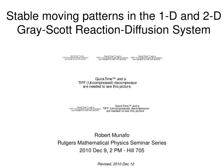
1. Stable moving patterns in the 1-D and 2-D Gray-Scott Reaction-Diffusion System Robert Munafo Rutgers Mathematical Physics Seminar Series 2010 Dec 9, 2 PM - Hill 705 Revised, 2010 Dec 12

2. Contents (outline of this talk) • Brief history, motivation and discovery • Methods and testing • New patterns and interactions (mostly video) • Connections; Open questions • Discussion

3. Brief History: Initial Motivation • 1994: Looking for a problem to run on new hardware • Supercomputer research led to Williams exhibit at Caltech (shown, left) • Literature was easy to find; problem was appealing • Exploring parameter space more closely Pearson “Complex patterns in a simple system” (Science261 1993) (illust. next slide) Lee et al. “Experimental observation of self-replicating spots in a reaction-diffusion system” (Nature369 1994) Ferrocyanide–iodate–sulphite reaction in gel reactor ( K4Fe(CN)6.3H2O, NaIO3 , Na2SO3 , H2SO4 , NaOH , bromothymol blue ) Roy Williams “Xmorphia” web exhibit (Caltech, 1994)

4. Brief Intro: Parameter Space Parameter space visualizations for several reaction-diffusion models, from fig. 3, Miyazawa et al. “Blending of animal colour patterns by hybridization” (Nature Comm.1(6) 2010) Parameter space and four pattern examples, from Pearson (ibid. 1993) Coloring imitates bromothymol blue pH indicator as in Lee et al. “Pattern formation by interacting chemical fronts” (Science261 1993): blue = low U; yellow = intermediate; red = high U

5. Brief History: 2009 Website Project • Denser coverage; explore more extreme parameter values Pearson: 34 sites; 0.045<k<0.066; 0.003<F<0.061; all static Williams: 45 sites; 0.032<k<0.066; 0.01<F<0.07; 4 video Munafo: 150+ sites; 0.03<k<0.072; 0.004<F<0.098 0.8 0.6 • Several types of starting patterns Parameter F 0.4 published work 0.2 • Video for each (k,F) point • Higher resolution and precision • Coloring to show both U and U/t • Describe and catalog all phenomena • Run each pattern “to completion” no matter how long that takes 0.3 0.4 0.5 0.6 0.7 Parameter k False color images: purple = lowest U, red = highest U, pastels = U/t > 0

6. * * New pattern types (2009) • Some type of exotic behavior at high F values was expected • Spirals were expected (seen in Belousov-Zhabotinsky and other reaction-diffusion systems) • k=0.061, F=0.062 has more diversity than all the rest put together • Also found: mixed spots and stripes; variations in branching; etc. k=0.059, F=0.09 k=0.057, F=0.09 * k=0.061, F=0.062 k=0.045, F=0.014 * Munafo (2009) www.mrob.com/pub/comp/xmorphia

7. F=0.08 red spot solitons F=0.06 solid blue state X stripes F=0.04 k=0.07 k=0.05 k=0.06 Inherent Instability k=0.062, F=0.06 Periodic boundary conditions; size 3.35w x 2.33h Each second is 1102 dtu Initial pattern of low-level random noise (0.4559<U<0.4562; 0.2674<V<0.2676) Final values: 0.35<U<0.90; 0.00<V<0.36 (approx.) (Contrast-enhanced images; lighter = higher U) t=3000 Turing-F600-k620.mp4 -- youtube.com/v/kXDTqqgrYCg t=3900 Gray-Scott parameter values for Turing instability (green; width to scale) and stable moving patterns (blue; width exaggerated). The video is at X • At many parameter values, patterns like this grow out of any inhomogeneity, no matter how small • This is not a consequence of numerical approximation error: proven by mathematical analysis. Dominant wavelength (spot size) depends on reaction dynamics and diffusion rate. Turing “The chemical basis of morphogenesis” (Phil. Trans. Royal Soc. London B237(641) 1952) t=4550 PDE4-20101127 Single 480x336 F 600 k 620 $ 4 % 9

8. How can we trust these results? Turing instability • Arbitrarily low-level noise can generate strong patterns • Instabilities can exist in the ideal (exact) system, and can be introduced by the numerical method • Complex patterns are already proven to be real • These new patterns are far more extraordinary • Mathematical proof/disproof probably impossible • How much precision is necessary? Is any finite precision sufficient for proof? • Is the standard precision “too accurate” to be relevant? The real world has known levels of quantization and randomness: “finite precision” • Goals: • Eliminate suspicion of numerical error • Quantify the sensitivity of these pattern phenomena to precision, randomness, reaction parameters and other environmental conditions Numerical instability Euler integration 4th-order Runge-Kutta

9. Verification Examples Two spots maintain the same distance while the pair rotates toward a 45° alignment • Two stable moving phenomena • One is clearly bogus, the other might be real U-shaped pattern moves at about 1 dlu per 62,000 dtu (dimensionless units of length, time) • Define something that is measurable • Model the sources of error, e.g.: measured value = true value + simulation error + measurement error simulation error = f(stability, precision, grid spacing, ...) CFL (Courant-Friedrichs-Lewy 1928) stability criterion (for the Laplacian term): Cx2/t (A higher value means greater stability. Constant C depends on e.g. k and F for the Gray-Scott system) • Progressively improve the simulation and look for a trend

10. Verification Procedure • Progressively improve x by √2 • Progressively improve CFL stability by √2 • Progressively improve t by needed amount (2√2) (amount of calculation increases by 4√2 each time: ratio of 1024 to 1 between “std” and “s4”) Expected Results: Movement is 100% spurious: measurements should tend towards zero If real, velocity should clearly converge on a nonzero value

11. Verification Examples - Results Suspect rotating 2-spot phenomenon cross-qtr. relative model max dU/dt interval velocity std 8.97e-7 5.6e5 1.0 s1.4 4.57e-7 1.12e6 0.50 s2 2.31e-7 2.18e6 0.26 s2.8 1.158e-7 4.34e6 0.129 s4 5.80e-8 8.7e6 0.064 • Two-spot pattern movement is bogus • Moving U-shaped pattern is real; Runge-Kutta gives little if any benefit • Asymptotic trends in values and in measurement errors, as expected Velocity of U-shaped pattern Limits on parameter k (when F=0.06) for stability of U-shaped pattern model dist pixels time velocity (meas.err) std 0.55418 79.2 35076 1/63294(45) s1.4 0.59863 121.1 37342 1/62379(64) s2 0.57042 163.1 35456 1/62159(27) s2.8 0.56947 230.3 35258 1/61913(44) s4 0.56553 323.5 35009 1/61905(12) model minimum maximum std 0.0608833 0.0609829 s1.4 0.0608796 0.0609831 s2 0.0608777 0.0609831 s2.8 0.0608767 0.0609830 s4 0.0608762 did not test measurement error in all values is +-1 in the last digit Same tests using 4th order Runge-Kutta model dist pixels time velocity (meas.err) std 0.57937 82.9 36559 1/63101 s1.4 0.56053 113.4 35021 1/62479 same s2 0.56351 161.2 35008 1/62124 as s2.8 0.56517 228.6 35003 1/61934 above s4 0.56574 323.6 35002 1/61870 2-spot data: Exploration Notes.txt, 20090422 Uskate velocities: 20101128 Min k: 20090422; max k: 20090415

12. Immunity to Noise • Pattern continues to move in the presence of noise, and generally behaves as expected of a real phenomenon • Similar tests (e.g. more frequent noise events each of lower amplitude) give similar results t=4700 t=64680 t=88500 k=0.0609, F=0.06 Periodic boundary conditions; size 3.35w x 2.33h 1 second  1100 dtu 4 U-shaped patterns traveling “up” Systematic noise perturbation applied once per 73.5 dtu Amplitude of each noise event starts at 0.001 and doubles every 11,000 dtu (10 seconds in this movie) At noise level 0.064, three patterns are destroyed; noise amplitude is then diminished to initial level (False-color: yellow = high U; pastel = positive U/t ) U-noise-immunity.mp4 -- youtube.com/v/_sir7yMLvIo PDE4-20101202 Single 480x336 F 600 k 609 % 10 cut and paste; 1e3nn; 2e3nn; 4e3nn; etc.

13. Symmetry-based Instability Tests k=0.0609, F=0.06 — Periodic boundary conditions; size 2.36w x 1.65h — Manually constructed initial pattern based on parts of naturally-evolved systems — 1 second = 265 dtu Two sets of three noise events; noise event amplitudes are 10-5, 0.001 and 0.1; pattern allowed to recover after each event Coloring (left image) same as before — Coloring (images below): white = positive U/t, black = negative U/t, shades of gray when magnitude of U/t is less than about 510-13 • Rotating and moving patterns have rotational or bilateral (resp.) symmetry which persists if the pattern is stable. • Instability and/or a return to symmetry are easier to observe in the derivative • Test static and linear-moving patterns at different angles to reveal influence by grid effects • Other tests include shifting parts of a pattern, applying noise to only part of a pattern, etc. • Such tests can reveal instability more quickly but do not prove stability. t=2850 t=38,000 t=1000 A pattern with an instability that this test does not help reveal Daedalus-stability.mp4 -- youtube.com/v/fWfsMVEeP5k PDE4-20101202 Single 480x336 F 600 k 609 3d load “s1.4-daedalus”; 1nn; 1e3nn; 1e5nn; 20c; etc.

14. Logarithmic Timebase, Long Duration • Some phenomena appear asymptotic to stability but actually keep moving forever • Running a simulation for as long as possible (currently >108 time units) and viewing the results at an exponentially accelerating speed can reveal some of these phenomena • Repulsion of solitons in 1-D (pictured, lower-right) has been studied mathematically for high ratios DU/DV (Doelman et al. “Slowly modulated two-pulse solutions...”, SIAM Jrl. on Appl. Math.61(3) 2000) with the result: (speed of movement) = Ae-Bt for positive constants A,B • There are many other phenomena in Gray-Scott systems that slow at similar rates t=78,125 t=1,250,000 Pair of solitons in 2-D system, k=0.068, F=0.042 Pair of solitons in 1-D system, k=0.0615, F=0.04 t=2107 t=3.2108 Eight solitons in a 2-D system, k=0.067, F=0.046

15. Discovery – Great Diversity • Part of routine scan for website exhibit project • “Negative solitons” (hereafter called “negatons”) exhibit attraction and multi-spot binding • Several types of patterns in one system • The “target” pattern is not stable at these parameter values, but is stable at the nearby parameters k=0.0609, F=0.06 Ordinary spot soliton (k=0.067, F=0.062) “negative soliton” (k=0.061, F=0.062) t=4770 t=47700 k=0.061, F=0.062 Periodic boundary conditions; size 3.35w x 2.33h 1 second  1190 dtu Initial pattern of a few randomly placed spots of relatively high U on a “blue” background (secondary homogeneous state, approx. U=0.420, V=0.293) (False-color: yellow = high U; pastel = positive U/t ) White curve = U; Black curve = V; dotted line shows cross-section taken Original-F620-k610-fr159.mp4 -- youtube.com/v/wFtXwFfrwWk “negative solitons” in Pearson (ibid. 1993) “Pattern ι is time independent and was observed for only a single parameter value.” (parameters unpublished, probably k=0.06, F=0.05) Intel PDE4-20090319 Single 480x336 F620 k609 s000 $0151 %1 m0159 M I

16. F=0.08 red X spot solitons F=0.06 solid blue state stripes  F=0.04 k=0.07 k=0.05 k=0.06 Discovery – Moving U Pattern • Moving “U” visible to right of center, short-lived (hits two negatons) • More unexpected negaton behavior: being “dragged” by other features t=125000 t=74200 t=8860 k=0.0609, F=0.062 Periodic boundary conditions; size 3.35w x 2.33h 1 second  3900 dtu Initial pattern and coloring same as before U-discovery-F620-k609-fr521.mp4 -- youtube.com/v/xGMuuPYhLiQ Original coloring -- youtube.com/v/ypYFUGiR51c This video is at X; Pearson’s type  is shown PPC PDE4-20090323 Single 480x336 F620 k609 s000 $0004 %1 m0521 M I

17. Long Duration TestDifferent Behaviors at Multiple Time Scales • First 30,000 dtu (40 seconds): blue spots grow to fill the space (a very common Gray-Scott behavior) • Up to 1.25 million dtu (75 seconds): complex behavior, double-spaced stripes, solitary negatons, etc. until all empty space is filled • Up to 6 million dtu (90 seconds): chaotic oscillation of parallel stripes growing, shrinking and twisting; gradually producing more spots • Sudden onset of stability: All chaotic motion ends (whole system drifts very slowly) t=1,780,000 t=441,000 t=2500 k=0.0609, F=0.062 Periodic boundary conditions; size 3.35w x 2.33h Initial pattern of spots (randomly chosen U<1, V>0) on solid red (U=1, V=0) background; coloring same as before Video uses accelerating time-lapse: simulation speed doubles every 6.7 seconds Exponential-time-lapse.mp4 -- youtube.com/v/-k98XOu7pC8 Intel PDE4-20090401 Single 480x336 F620 k609 s000 $0027^ %3 m1248 M I

18. Complex Interactions • U-shape can influence other objects and survive (although it generally does not) • The clusters of negatons along the top move and rotate, very slowly t=280,000 T=120,000 t=60,000 k=0.0609, F=0.06 Periodic boundary conditions; size 3.35w x 2.33h Each second is 10,000 dtu Manually constructed initial pattern based on parts of naturally-evolved systems Coloring same as before complex-interactions-1.mp4 -- youtube.com/v/hgTBOf7gg8E PDE4-20101202 Single 480x336 F 600 k 609 load “cplx-4”; cut and paste negatons; etc.

19. Slow Movement, Rotation • There are many very slow patterns; a few of the more common are shown here • The “target” (negaton with annulus) is a common product of spotlike initial patterns, and adjacent negatons typically make it move or rotate • The 4 negatons left by the collision of two U patterns are in an unstable equilibrium T=7,000,000 T=1,500,000 t=0 k=0.0609, F=0.06 Periodic boundary conditions; size 3.35w x 2.33h Each second is 100,000 dtu Manually constructed initial pattern based on parts of naturally-evolved systems Coloring same as before slow movers and rotaters.mp4 -- youtube.com/v/PB3lPMhwIo0 Stability analysis of another slow-rotating pattern Stability testing of 4-negaton pattern; stable form shown at right PDE4-20101202 Single 480x336 F 600 k 609 load “target-3x2-lopsided”; cut and paste negatons and Us; etc.

20. A Gray-Scott Pattern Bestiary • Almost everything that keeps its shape moves indefinitely • In general, a pattern will: • move in a straight line, if is has (only) bilateral symmetry • rotate, if it has (only) rotational symmetry • move on a curved path, if it has no symmetry at all • Lone negatons are frequently “captured” and/or “pushed” by a moving pattern (unstable) k=0.0609, F=0.06 Contrast-enhanced grayscale, lighter = higher U Most patterns were manually constructed from parts of naturally occurring forms Note: Many of these are not yet thoroughly tested

21. Relation to Other Work:“Negaton” Clusters and Targets * • Spots and “target” patterns very similar to the Gray-Scott “negatons” are seen in papers by Schenk, Purwins, et al. • In a 1998 work, a 2-component R-D system is studied; the spots are stationary and are reported to “bind” into stable groupings with specific geometrical configurations (as shown). There are differences between this system and Gray-Scott, evident in which “molecules” are reported as stable. • In a 1999 work (by Schenk alone) a 3-component R-D system includes a “target” pattern with a very similar cross-section. * From Schenk et al. “Interaction of self-organized quasiparticles...” (Physical Review E57(6) 1998), fig. 1 and 5 The pattern marked*is stable in Gray-Scott at {k=0.0609, F=0.06}, the pattern marked is * not. Target pattern in Gray-Scott, k=0.0609, F=0.06, with U and V levels at cross-section through center Target pattern from C. P. Schenk (PhD dissertation, WWU Münster, 1999) p. 116 fig. 4.37

22. Relation to Other Work: Halos • The light and dark “rings” or “halos” are seen in physical experiments and numerical simulations intended to model both physical and biological systems • When spots appear in these systems, as in Gray-Scott, the spots tend to be seen at certain “quantized” distances • Halo amplitudes, spot spacings and relative sizes differ; this also reflects changes seen in Gray-Scott as the k and/or F parameters are changed Negatons with halos (Gray-Scott system, k=0.0609, F=0.06, lighter = higher U; exaggerated contrast) Spots with halos in numerical simulation by Barrio et al. “Modeling the skin patterns of fishes” (Physical Review E79 031908 2009) fig. 11 Spots with halos in gas-discharge experiment by Lars Stollenwerk (“Pattern formation in AC gas discharge systems”, website of the Institute of Applied Physics, WWU Münster, 2008) fig. 3d Halos also appear in models by Schenk, Purwins, et al (ibid., 1998 and 1999, shown elsewhere) in work related to gas discharge experiments

23. One-Dimensional Gray-Scott Model • There are extensive results on the 1-D system based on rigorous mathematical analysis (most are for higher ratios DU/DV than in the systems presented here) • The “spiral wavefront” observed at many parameter values in the 2-D system is also a viable self-sustaining stable moving pattern in the 1-D system at the same parameter values • For many parameter values that support “negative stripes” in the 2-D system, certain asymmetrical clumps of “negatons” form stable moving patterns in the 1-D system • Negatons in 1-D were reported (shown) as early as 1996 2-D spirals and 1-D pulse at k=0.047, F=0.014 Single 1-D negaton inside a growing region of solid “blue state” at k=0.06, F=0.05, from Mazin et al. “Pattern formation in the bistable Gray-Scott model” (Math. and Comp. in Simulation40 1996) fig. 9 Representative 2-D and 1-D patterns at k=0.0609, F=0.06 (Note: Non-existence results of Doelman, Kaper and Zegeling (1997) and of Muratov and Osipov (2000) are not applicable because they concern models with a much higher ratio DU/DV ) (Note: 2-D spirals shown here, and observed at many combinations of k and F parameter values, were not reported by Pearson (ibid. 1993). This is likely because of Pearson’s starting pattern, not because spirals would break up as claimed by Muratov and Osipov (2000) p. 84)

24. Open Questions • Why does the U-shaped pattern move and keep its shape? • As parameter k is increased, leading end of double-stripe (shown) moves faster, but trailing end moves slower and the object lengthens; in the other direction (decreasing k) the reverse is true • When these two speeds are closely matched, the U shape (shown) neither grows nor shrinks – why? • Do these patterns appear in other reaction-diffusion models? • Universal presence of other pattern types suggests this; parameter space maps should make it easy to find; nearby Turing effect is possibly relevant • Can any of the special properties of these patterns be proven mathematically? • 1-D systems seem particularly well suited to this task • Shape of negaton “halos” is easy to solve • Most existing work applies conditions or limits that exclude the commonly studied DU/DV=2 systems Double-stripe and U From Miyazawa (ibid. 2010) 1-D moving pattern

25. Discussion Robert Munafo mrob.com/sci mrob.com/pub/comp/xmorphia mrob27(at)gmail.com 617-335-1321