Download
1 / 55
560 likes | 624 Views
Jordi Cortadella, Universitat Politecnica de Catalunya, Barcelona Mike Kishinevsky, Intel Corp., Strategic CAD Labs, Hillsboro. Elasticity and petri nets. Moore’s law. Source: Intel Corp. Is the GHz race over ?. Many-Core is here. Source: Intel Corp. Why this tutorial ?.

E N D
Jordi Cortadella, Universitat Politecnica de Catalunya, Barcelona Mike Kishinevsky, Intel Corp., Strategic CAD Labs, Hillsboro Elasticity and petri nets
Moore’s law Source: Intel Corp.
Many-Core is here Source: Intel Corp.
Why this tutorial ? • Digital circuits are complex concurrent systems • Variability and power consumption are key critical aspects in deep submicron technologies • Multi (many)-core systems will become a novel paradigm: • System design • Applications • Concurrent programming • Theory of concurrency may play a relevant role in this new scenario
Elasticity • Tolerance to delay variability • Different forms of elasticity • Asynchronous: no clock • Synchronous: variability synchronized with a clock • In all forms of elasticity, token-based computations are performed(req/ack, valid/stop signals are used)
Outline • Asynchronous elastic systems • The basics: circuits and elasticity • Synthesis of asynchronous circuits from Petri nets • Modern methods for the synthesis of large controllers • De-synchronization: from synchronous to asynchronous • Synchronous elastic systems • Basics of synchronous elastic systems • Early evaluation and performance analysis • Optimization of elastic systems and their correctness
Outline Gates, latches and flip-flops.Combinational and sequential circuits. Basic concepts on asynchronous circuit design. Petri net models for asynchronous controllers. Signal Transition Graphs.
Boolean functions Composed from logic gates a x b a y b a b z c d
Memory elements: latches Q Q D D L H En En Active low: En = 1 (opaque): Q = prev(Q) En = 0 (transparent): Q = D Active high: En = 0 (opaque): Q = prev(Q) En = 1 (transparent): Q = D
Memory elements: flip-flop Q D Q L H D FF CLK CLK CLK D Q
Finite-state automata Inputs Ouputs CL STATE • Output function • Next-state function CLK
Network of Computing Units Out In B3 B1 B2 No combinational cycles
Marked Graph Model Circuit Register Combinational logic Marked graph
Outline • What is an asynchronous circuit ? • Asynchronous communication • Asynchronous design styles (Micropipelines) • Asynchronous logic building blocks • Control specification and implementation • Delay models and classes of async circuits • Channel-based design • Why asynchronous circuits ?
R CL R CL R CL R CLK Synchronous circuit Implicit (global) synchronization between blocks Clock period > Max Delay (CL + R)
Asynchronous circuit Ack R CL R CL R CL R Req Explicit (local) synchronization: Req / Ack handshakes
Motivation for asynchronous • Asynchronous design is often unavoidable: • Asynchronous interfaces, arbiters etc. • Modern clocking is multi–phase and distributed –and virtually ‘asynchronous’ (cf. GALS – next slide): • Mesachronous (clock travels together with data) • Local (possibly stretchable) clock generation • Robust asynchronous design flow is coming(e.g. VLSI programming from Philips, Balsa fromUniv. of Manchester, NCL from Theseus Logic …)
Globally Async Locally Sync (GALS) Asynchronous World Clocked Domain Req3 Req1 R R CL Ack3 Ack1 Local CLK Req4 Req2 Ack4 Ack2 Async-to-sync Wrapper
Key Design Differences • Synchronous logic design: • proceeds without taking timing correctness(hazards, signal ack–ing etc.) into account • Combinational logic and memory latches(registers) are built separately • Static timing analysis of CL is sufficient todetermine the Max Delay (clock period) • Fixed set–up and hold conditions for latches
Key Design Differences • Asynchronous logic design: • Must ensure hazard–freedom, signal ack–ing,local timing constraints • Combinational logic and memory latches (registers) are often mixed in “complex gates” • Dynamic timing analysis of logic is needed to determine relative delays between paths • To avoid complex issues, circuits may be builtas Delay-insensitive and/or Speed-independent (as discussed later)
Synchronous communication • Clock edges determine the time instants where data must be sampled • Data wires may glitch between clock edges(set–up/hold times must be satisfied) • Data are transmitted at a fixed rate(clock frequency) 1 1 0 0 1 0
Dual rail 1 1 1 • Two wires with L(low) and H (high) per bit • “LL” = “spacer”, “LH” = “0”, “HL” = “1” • n–bit data communication requires 2n wires • Each bit is self-timed • Other delay-insensitive codes exist (e.g. k-of-n)and event–based signalling (choice criteria: pin and power efficiency) 0 0 0
Bundled data • Validity signal • Similar to an aperiodic local clock • n–bit data communication requires n+1 wires • Data wires may glitch when no valid • Signaling protocols • level sensitive (latch) • transition sensitive (register): 2–phase / 4–phase 1 1 0 0 1 0
Example: memory read cycle Valid address • Transition signaling, 4-phase Address A A Valid data Data D D
Example: memory read cycle Valid address • Transition signaling, 2-phase A A Address Valid data Data D D
Asynchronous modules DATA PATH Data IN Data OUT • Signaling protocol: reqin+ start+ [computation] done+ reqout+ ackout+ ackin+reqin- start- [reset] done- reqout- ackout- ackin-(more concurrency is also possible) start done req in req out CONTROL ack in ack out
A C Z B A B Z+ 0 0 0 0 1 Z 1 0 Z 1 1 1 Asynchronous latches: C element Vdd A B Z B A Z B A Z Static Logic Implementation A B [van Berkel 91] Gnd
Vdd A B Z B A Gnd C-element: Other implementations Vdd A Weak inverter B Z B A Dynamic Quasi-Static Gnd
A.t C.t B.t A.f C.f B.f Dual-rail logic Dual-rail AND gate Valid behavior for monotonic environment
done C Completion detection tree Completion detection Dual-rail logic • • • • • •
Differentialcascodevoltageswitchlogic start Z.f Z.t done A.t N-type transistor network C.f B.f A.f B.t C.t start 3–input AND/NAND gate
Example of dual-rail design • Asynchronous dual-rail ripple-carry adder(A. Martin, 1991) • Critical delay is proportional to logN(N=number of bits) • 32–bit adder delay (1.6m MOSIS CMOS): 11 ns versus 40 ns for synchronous • Async cell transistor count = 34versus synchronous = 28
start done delay Bundled-data logic blocks Single-rail logic • • • • • • Conventional logic + matched delay
r1 g1 C d1 r2 g2 d2 r1 a1 r a r2 a2 sel outf in outt Micropipelines(Sutherland 89) Micropipeline (2-phase) control blocks Request-Grant-Done (RGD)Arbiter Join Merge out0 in out1 Select Toggle Call
C C C delay delay delay Micropipelines (Sutherland 89) Aout Ain C L logic L logic L logic L Rin Rout
Data-path / Control L logic L logic L logic L Rin Rout CONTROL Ain Aout
Control specification A+ A B+ B A– A input B output B–
Control specification A+ B– B A A– B+
C Control specification A+ B+ A C+ C B A– B– C–
C Control specification A+ B+ A C+ C A– B B– C–
Ro+ Ri+ Ri Ro FIFO cntrl Ao+ Ai+ Ao Ai Ro- Ri- C C Ai- Ao- Ri Ro Ao Ai Control specification
A simple filter: specification IN Ain Rin y := 0; loop x := READ (IN); WRITE (OUT, (x+y)/2); y := x; end loop filter Aout Rout OUT
+ OUT x y IN Ry Ay Rx Ax Ra Aa Rin Rout control Ain Aout A simple filter: block diagram • x and y are level-sensitive latches (transparent when R=1) • + is a bundled-data adder (matched delay between Ra and Aa) • Rin indicates the validity of IN • After Ain+ the environment is allowed to change IN • (Rout,Aout) control a level-sensitive latch at the output
+ OUT x y IN Ry Ay Rx Ax Ra Aa Rin Rout control Ain Aout Rout+ Ra+ Ry+ Rx+ Rin+ Aout+ Aa+ Ay+ Ax+ Ain+ Rout– Ra– Ry– Rx– Rin– Aout– Aa– Ay– Ax– Ain– A simple filter: control spec.
Rx Ax Aa Ry Ra Ay Aout C Ain Rout Rin Rout+ Ra+ Ry+ Rx+ Rin+ Aout+ Aa+ Ay+ Ax+ Ain+ Rout– Ra– Ry– Rx– Rin– Aout– Aa– Ay– Ax– Ain– A simple filter: control impl.
x’ z+ x– x y z’ z x+ y+ z– y– Taking delays into account • Delay assumptions: • Environment: 3 time units • Gates: 1 time unit events: x+ x’– y+ z+ z’– x– x’+ z– z’+ y– time: 3 4 5 6 7 9 10 12 13 14