Using Statistics To Make Inferences 8
790 likes | 1.05k Views
Using Statistics To Make Inferences 8. Summary Contingency tables. Goodness of fit test. 1. Sunday, 10 August 2014 11:52 AM. Goals. To assess contingency tables for independence. To perform and interpret a goodness of fit test. Practical Construct and analyse contingency tables. 2.

Using Statistics To Make Inferences 8
E N D
Presentation Transcript
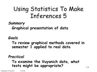
Using Statistics To Make Inferences 8 Summary Contingency tables. Goodness of fit test. 1 Sunday, 10 August 201411:52 AM
Goals To assess contingency tables for independence. To perform and interpret a goodness of fit test. Practical Construct and analyse contingency tables. 2
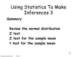
Recall To compare a population and sample variance we employed? χ2 Cc cc 3
Today The probability approach from last week is employed to tell if “observed” data confirms to the pattern “expected” under a given model. 4
Categorical Data - Example Assessed intelligence of athletic and non-athletic schoolboys. K. Pearson “On The Relationship Of Intelligence To Size And Shape Of Head, And To Other Physical And Mental Characters”, Biometrika, 1906, 5, 105-146, data on page 144. 5
Procedure • Formulate a null hypothesis. Typically the null hypothesis is that there is no association between the factors. • Calculate expected frequencies for the cells in the table on the assumption that the null hypothesis is true. • Calculate the chi-squared statistic. This is for an r x c table with entries in row i and column j. 6
Procedure • Compare the calculated statistic with tabulated values of the chi-squared distribution with ν degrees of freedom. ν = (rows ‑ 1)(columns ‑ 1) = (r – 1)(c – 1) 7
Key Assumptions • Independence of the observations. The data found in each cell of the contingency table used in the chi-squared test must be independent observations and non-correlated. 2. Large enough expected cell counts. As described by Yates, et al., "No more than 20% of the expected counts are less than 5 and all individual expected counts are 1 or greater" (Yates, Moore & McCabe, 1999, p. 734). 8
Key Assumptions • Randomness of data. The data in the table should be randomly selected. 4. Sufficient Sample Size. It is also generally assumed that the sample size for the entire contingency table is sufficiently large to prevent falsely accepting the null hypothesis when the null hypothesis is true. 9
Example Assessed intelligence of athletic and non athletic schoolboys. Observed 10
Probabilities C C C C C C C C C C C C C C C The probability a random boy is athletic is The probability a random boy is bright is Assuming independence, the probability a random boy is both athletic and bright is For 1708 respondents the expected number of athletic bright boys is 11
Expected The expected number of athletic bright boys is 12
Expected The expected number of athletic stupid boys is 13
Expected The expected number of athletic stupid boys is 1148 – 530.98 = 617.02 14
Expected The expected number of lazy bright boys is 15
Expected The expected number of stupid lazy boys is 16
Expected The expected number of stupid lazy boys is 918 – 617.02 = 300.98 17
Expected 18
χ2 Observed Expected 19
χ2 As a general rule to employ this statistic, all expected frequencies should exceed 5. If this is not the case categories are pooled (merged) to achieve this goal. See the Prussian data later. 20
Conclusion The result is significant (26.73 > 3.84) at the 5% level. So we reject the hypothesis of independence between athletic prowess and intelligence. 21
SPSS Raw data Note v1 are the row labels v2 are the column labels v3 is the frequency for each cell 22
SPSS Data > Weight Cases Since frequency data has been input, necessary to weight. This is essential, do not use percentages. 23
SPSS Analyze > Descriptive Statistics > Crosstabs Set row and column variables. Frequencies already set. 24
SPSS Select chi-square 25
SPSS Select Observed – input data Expected – output data, under the model 26
SPSS Expected cell frequencies Expected under the model. 27
SPSS Pearson Chi Square is the required statistic ff Do not report p = .000, rather p < .001 Note Fisher’s exact test, only available in SPSS for 2x2 tables (see next slide). 28
What If We Have Small Cell Counts? Fisher's exact test The Fisher's exact test is used when you want to conduct a chi-square test but one or more of your cells has an expected frequency of five or less. Remember that the chi-square test assumes that each cell has an expected frequency of five or more, but the Fisher's exact test has no such assumption and can be used regardless of how small the expected frequency is. In SPSS, unless you have the SPSS Exact Test Module, you can only perform a Fisher's exact test on a 2x2 table, and these results are presented by default. 29
Aside Two dials were compared. A subject was asked to read each dial many times, and the experimenter recorded his errors. Altogether 7 subjects were tested. The data shows how many errors each subject produced. Do the two conditions differ at the 0.05 significance level (give the appropriate p value)? Observed data 1 2 3 4 5 6 7 36 31 31 29 32 25 26 29 35 34 35 34 35 30 What key word describes this data? 30
Aside C C C C C C C C C c What tests are available for paired data? One sample t test Sign test Wilcoxon Signed Ranks Test 31
Aside What tests are available for paired data? What assumptions are made? normality One sample t test Sign test No assumption of normality Wilcoxon Signed Ranks Test Resembles the SignTest in scope, but it is much more sensitive. In fact, for large numbers it is almost as sensitive as the Student t-test 32
Aside What tests are available for paired data? One sample t test Wilcoxon Signed Ranks Test Sign test Sign test answers the question How Often?, whereas other tests answer the question How Much? One sample t test – mean Wilcoxon Signed Ranks Test - median 33
Example The table is based on case-records of women employees in Royal Ordnance factories during 1943-6. The same test being carried out on the left eye (columns) and right eye (rows). Stuart “The estimation and comparison of strengths of association in contingency tables”, Biometrika, 1953, 40, 105-110. 34
Observed Is there any obvious structure? 35
Expected In general to find the expected frequency in a particular cell the equation is Row total x Column total / Grand total 36
Expected In general to find the expected frequency in a particular cell the equation is Row total x Column total / Grand total So for highest right and left the equation becomes 1976 x 1907 / 7477 = 503.98 37
Expected Row total x Column total / Grand total 1976 x 1907 / 7477 = 503.98 38
Expected Row total x Column total / Grand total 39
Expected The missing values are simply found by subtraction 40
Expected 1976 – 503.98 – 587.22 – 662.54 = 222.26 41
Expected 1976 – 503.98 – 587.22 – 662.54 = 222.26 42
Expected Similarly for the remaining cells 43
Expected 44
Short Cut Contributions to the χ2 statistic, for the top left cell the contribution is 45
Conclusion The above statistic makes it very clear that there is some relationship between the quality of the right and left eyes. 46
Total χ2 47
Conclusion The above statistic makes it very clear that there is some relationship between the quality of the right and left eyes. 48
SPSS Raw data 49
SPSS Expected cell frequencies 50