Download
1 / 29
290 likes | 458 Views
Thermo-hydraulic simulation of the ITER PF coil joints based on their coupling losses calculated with JackPot-AC. Ezra van Lanen 1 , Wietse Offringa 1 , Yuri Ilin 2 and Arend Nijhuis 1 1 Energy, Materials and Systems, Enschede, the Netherlands 2 ITER organisation, Cadarache, France

E N D
Thermo-hydraulic simulation of the ITER PF coil joints based on their coupling losses calculated with JackPot-AC Ezra van Lanen1, Wietse Offringa1, Yuri Ilin2 and Arend Nijhuis1 1Energy, Materials and Systems, Enschede, the Netherlands 2ITER organisation, Cadarache, France CHATS-AS workshop, CERN, October 2011 Service Contract No.: UT- ITER/CT/09/4300000070
Outline Objective for temperature calculation JackPot-AC coupling loss model Hysteresis loss model Thermal model Results Conclusions
Outline Objective for temperature calculation JackPot-AC coupling loss model Hysteresis loss model Thermal model Results Conclusions
Temperature calculation workflow • Coupling loss model has only linear components; no strand saturation is included; • As a result, the temperature distribution is not calculated simultaneously, but afterwards; • The algorithm is as follows: • Calculate coupling losses, no saturation in strands • If strand currents exceed their critical current, it is assumed that a quench will happen anyway; • Calculate the magnetic field at strand locations; • Calculate the critical current assuming constant temperature • First opportunity for checking instability; • Calculate hysteresis loss (requires critical current) • Calculate temperature distribution (and if necessary, calculate the critical current again based on this temperature)
Outline Objective for temperature calculation JackPot-AC coupling loss model Hysteresis loss model Thermal model Results Conclusions
Overview of JackPot-AC network model Cable cross section from JackPot simulation Simplified electrical network • Cable model that accurately describes all strand trajectories in CICC; • Simulated strand trajectories are used to: • Calculate interstrand contact resistance distribution; • Strand-to-joint’s copper sleeve contact resistance distribution; • Mutual inductances • Coupling with background field
Overview of JackPot-AC copper sole model A Partial Element Equivalent Circuit (PEEC) model is used to simulate the copper sole; This results in an electrical network that can easily be coupled to the cable model; The shape of the sole is approximated by removing PEEC boxes at the cable locations The coupling between the voltage nodes of the copper sole and the strands is determined from the geometric data; Similar to the interstrand resistances, the strand-to-sole resistances depend on the contact area between strands and the cable periphery.
Validation JackPot-AC joint coupling loss model Serial field Parallel field The joint model has been validated with measurements on a mock-up joint; Interstrand and strand-to-joint contact resistivity were determined from interstrand resistance measurements on sub-size CICCs; Additional measurements were carried out on one cable and the copper sole separately; The measurements were done with different orientation of the harmonic background field.
Validation JackPot-AC joint coupling loss model Serial field Parallel field Good agreement between measurement and simulation; Expected deviation due to hysteresis loss and intra-strand loss in the measurements, which are not included in the model; Peak power dissipation in “parallel” field at much lower frequency than in “serial” field due to the inter-cable coupling loops.
Simulation conditions for an ITER PF joint • Three locations for the joints are used; • The radial field components are stronger in the “Top” and “Bottom” joints than in the “Middle” joint; • Transport current distribution among strands is assumed homogeneous at current entry and exit; • To allow for current distribution among strands outside the joint region, an extra 0.25 m of cable is added at both ends of the joint in the simulation. • The joint RRR is 100.
Coupling loss in the PF2-top joint at the start of a 15 MA plasma scenario A 300 second linear coil current ramp precedes the start of the plasma scenario (left figure); This is included in the simulations to have an initial current distribution; The power dissipation includes both the effects of dB/dt and of the transport current.
Strand currents in PF2-top Cable 1 The left figure shows the strand currents of Cable 1 in the centre of the joint versus time; The clear bias towards negative values is caused by inter-cable coupling currents due to the radial field component; It’s effect is made clear by the right figure, which shows the total cable current along the length of the two cables at t = 25 seconds.
Outline Objective for temperature calculation JackPot-AC coupling loss model Hysteresis loss model Thermal model Results Conclusions
Hysteresis model • The model assumes full filament penetration during the whole campaing. In general, the penetration field is only a few tenths of teslas; • The equations for calculating the transient hysteresis loss are • Ic = critical current • It = transport current • deff = effective filament diameter • knonCu = fraction of non-copper material • This includes both the change of the background field and the change of the transport current
Hysteresis loss in PF5-middle Cable 1 at start of scenario Joint region • In the cable region the field on the strands is either amplified or reduced due to the transport current (-0.5 < axis < -0.25 meter); • As a result, the hysteresis loss alternates along the length; • Inside the joint, the transport current decays; the hysteresis loss becomes more homogeneous
Outline Objective for temperature calculation JackPot-AC coupling loss model Hysteresis loss model Thermal model Results Conclusions
Overview of thermal model • The temperature distribution is calculated along the length of the joint for: • Individual strand bundles of both cables • Helium inside these bundles • Upper and lower half of the joint box • Thus, for PF joints, a total of 26 temperature profiles are calculated
Equations for the strand bundle Heat exchange with helium Heat exchange with sole Power dissipation in strand bundle • The density (rst), heat transfer coefficient (hst-He), strand-helium wetted perimeter (Cst) and heat conductivity (kst) are assumed constant; • A quadratic fit for the cp,st (specific heat) versus temperature is taken; • Direct heat exchange between strand bundles does not take place; • This exchange is covered by the helium; • Contact term is a function of position to account for the rotation of the petal, and the partial contact between the cable and the copper sole.
Equations for the copper sole Heat exchange with helium Heat exchange with other half of sole Power dissipation in strand bundle The density (rCu), heat transfer coefficients (hsole-He and hsole-sole), joint-helium wetted perimeter (Csole) and heat conductivity (kCu) are assumed constant; A quadratic fit for the cp,sole (specific heat) versus temperature is taken;
Equations for the helium flow • The heat transfer coefficient (hHe-He) inter-petal wetted perimeter (CHe_He) are assumed constant; • Linear interpolation is used from data for the density (rHe) and specific heat (cp,He) versus temperature relationship; • A fixed mass flow rate ( ) is assumed • Pressure is 5 bar. Helium flow Heat exchange with cable Heat exchange with sole Heat exchange with other petals
Outline Objective for temperature calculation JackPot-AC coupling loss model Hysteresis loss model Thermal model Results Conclusions
PF5: Power dissipation along joint length The power dissipation is calculated along the length of each component (strand bundle, joint half) Shown here is the result at the start of the plasma scenario (t = 0 s); CJ = cable-to-joint contact layer; Biased power due to coupling currents between cables
PF5-top: Petal temperature distribution at start of scenario Results at start of the scenario (t = 0 s); Despite biased power dissipation, the temperature profiles are equivalent in both cables; Periodicity of the temperature is due to the rotation of the cable in the joint and periodic contact with the copper sole.
PF5-top: Copper sole temperature Results at start of the scenario (t = 0 s); Temperature profile identical for both joint halfs; High thermal conductivity leads to smoothing of the temperature distribution; Considerably higher temperature in the copper sole than in the cables.
PF5: Evolution of temperature during the scenario Start of plasma Plasma burn phase The temperature is shown at the downstream-end of the “hottest” petal (identical geometries were taken for the “top” and “middle” joints); The stronger radial field in the “top” joint leads to a +0.15 K higher temperature after the start of plasma; This temperature difference decays during the plasma burn phase, when the dB/dt and dI/dt are much smaller.
Performance of other joints Other joints have been simulated as well, which show similar temperature behaviour during the plasma scenario; The PF6-bottom joint shows a large temperature increase during the current ramp preceding the scenario; During the scenario, its temperature decreases, whereas the transport current increases…
PF6-bottom: Inter-cable coupling currents The PF6 coil starts the scenario with a high transport current; As a result, it also has a high dB/dt during this phase, with a considerable radial component for the bottom joint; This results in much larger coupling currents before the scenario (left figure) than during the scenario (right figure).
Outline Objective for temperature calculation JackPot-AC coupling loss model Hysteresis loss model Thermal model Results Conclusions
Conclusions JackPot-AC, The coupling loss model for CICC joints has been expanded with a thermal model; Although these models are not coupled, they serves as a powerful analysis tool for CICC joints; The copper sole smears out non-uniform power dissipation along the cable axes; The radial field component causes a considerable coupling current between the cables in joints at the edges of a coil, compared to joints in the middle; As a result of these coupling currents, a more than 0.15 K peak temperature difference is observed in the simulation of the PF5 joints; Similar coupling currents increase the peak temperature of the PF6 bottom joint to more than 0.35 K above the inlet temperature before the start of the plasma scenario.