Download
1 / 34
370 likes | 610 Views
Emission mechanisms. I . Giorgio Matt (Dipartimento di Fisica, Università Roma Tre, Italy) Reference: Rybicki & Lightman, “Radiative processes in astrophysics”, Wiley. Outline of the lecture . Basics (emission, absorption, radiative transfer) Bremsstrahlung Synchrotron emission

E N D
Emission mechanisms. I GiorgioMatt (Dipartimento di Fisica, Università Roma Tre, Italy) Reference: Rybicki & Lightman, “Radiative processes in astrophysics”, Wiley
Outline of the lecture • Basics (emission, absorption, radiative transfer) • Bremsstrahlung • Synchrotron emission • Compton Scattering (Inverse Compton)
Any charged particle in accelerated motion emits e.m. radiation. The intensity of the radiation is governed by Larmor’s formulae: where q is the electric charge, v the particle velocity,Θ the angle between the acceleration vector and the direction of emission ( Averaged over emission angles) • The power is in general inversely proportional to the square of the mass of the emitting particle !!(dv/dt = F/m) Electrons emit much more than protons !
The previous formulae are valid in the non relativistic case. If the velocity of the emitting particle is relativistic, then the formula for the angle-averaged emission is: where γ is the Lorenzt factor ( γ=(1-v2/c2)-1/2) of the emitting particle, and the acceleration vector is decomposed in the components parallel and perpendicular to the velocity. Of course, for γ~1 the non relativistic formula is recovered.
The equation of radiative transfer is: If matter is in local thermodynamic equilibrium, Sν is a universal function of temperature: Sν = Bν(T)(Kirchoff’s law). Bν(T) is the Planck function:
Polarization The polarization vector (which is a pseudovector, i.e. modulus π) rotates forming an ellipse. Polarization is described by the Stokes parameters: If V=0, radiation is linearly polarized If Q=U=0, radiation is circularly polarized
Polarization Summing up the contributions of all photons, I increases while this is not necessarily so for the other Stokes parameters. Therefore: The net polarization degree and angle are given by:
Black Body emission If perfect thermal equilibrium between radiation and matter is reached throughout the material, Iν is independent of τ. In this case the matter emits as a Black Body:
Black body emission occurs when τ→∞, so in practice there are always deviations from a pure Black Body spectrum due to finite opacities and surface layers effects. The only perfect Black Body is the Cosmic Microwave Background radiation.
Thomson scattering It is the interaction between a photon and an electron (at rest), with hν«mc2. It is an elastic process. The cross section is: The differential cross section is: The scattered radiation is polarized. E.g., the polarization degree of a parallel beam of unpolarized radiation is:
Pair production and annihilation A e+-e- pair may annihilate producing two γ-rays (to conserve momentum). If the electrons are not relativistic, the two photons have E=511 keV. Conversely, two γ-rays (or a γ-ray with the help of a nucleus) may produce a e+-e- pair Pair production is of course a threshold process. Eγ1 Eγ2 > 2m2c4 The pair production cross sections are: γ-rays interacts with IR photons. The maximum distance at which an extragalactic γ-ray source is observed provides an estimate of the (poorly known) cosmic IR background
Bremsstrahlung (“braking radiation”) a.k.a. free-free emission It is produced by the deflection of a charged particle (usually an electron in astrophysical situations) in the Coulombian field of another charged particle (usually an atomic nucleus). Also referred to as free-free emission because the electron is free both before and after the deflection.
b is called the impact parameter The interaction occurs on a timescale Δt ≈ 2b/v A Fourier analysis leads to the emitted energy per unit frequency in a single collision, which is inversely proportional to the square of: the mass, velocity of the deflected particle (electron) and impact parameter.
Integrating over the impact parameter, we obtain: bmaxand bminmust be evaluated taking into account quantum mechanics. They are calculated numerically. gffis the so calledGaunt factor. It is of order unity for large intervals of the parameters. To get the final emissivity, we have to integrate over the velocity distribution of the electrons.
Thermal Bremsstrahlung If electrons are in thermal equilibrium, their velocity distribution is Maxwellian. The bremsstrahlung emission thus becomes: Integrated over frequencies Emission measure The above formulae are valid in the optically thin case. If τ >> 1, we of course have the Black Body emission
Free-free absorption A photon can be absorbed by a free electron in the Coulombian field of an atom: it is the free-free absorption, which is the aborption mechanism corresponding to bremsstrahlung. Thus, for thermal electrons: At low frequencies matter in thermal equilibrium is optically thick to free-free aborption, becoming thin at high frequencies.
Polarization Bremsstrahlung photons are polarized with the electric vector perpendicular to the plane of interaction. In most astrophysical situations, and certainly in case of thermal bremsstrahlung, the planes of interaction are randomly distributed, resulting in null net polarization. For an anisotropic distribution of electrons, however, bremsstrahlung emission can be polarized.
Cooling time For any emission mechanism, the cooling time is defined as: where E is the energy of the emitting particle and dE/dt the energy lost by radiation. For thermal bremsstrahlung: • Radio image of the Orion Nebula X-ray emission of the Coma Cluster The cooling time is of order one thousand years for a HII regions, and of a few times 1010 years (i.e. more than the age of the Universe) for a Cluster of galaxies
Synchrotron emission It is produced by the acceleration of a moving charged particle in a magnetic field due to the Lorentz force: The force is always perpendicular to the particle velocity, so it does not do work. Therefore, the particle moves in a helical path with constant |v| (if energy losses by radiation are neglected). The radius of gyration and the frequency of the orbit are ( is the angle between v and B):
Let us assume the charged particle is an electron. Using the relativistic Larmor formulae, and averaging over , the power emitted by an electron is (β≡v/c): The synchrotron spectrum from a single electron is peaked at:
To get the total spectrum from a population of electrons, we must know their energy distribution. A particularly relavant case is that of a power law distribution,N(E)=KE-p. The total spectrum is also a power law, F(ν)=Cν-, with =(p-1)/2 F(ν)=A(p)KB(p+1)/2ν-
Synchrotron self-absorption If the energy distribution of the electrons is non-thermal, e.g. a power law, N(E)=KE-p, the absorption coefficient cannot be derived from the Kirchhoff’s law. The direct calculation using Einstein’s coefficient yields: In the optically thick region, the spectrum is independent of p The transition frequency is related to the magnetic field and can be used to determine it.
Polarization The radiation is polarized perpendicularly to the projection of B on the plane of the sky For a power law distribution of emitting particles, the degree of polarization is Π=(p+1)/(p+7/3). This is actually un upper limit, because the magnetic field is never perfectly ordered.
(Electron’s rest mass is irreducible) Cooling time The cooling time is: For the interstellar matter (B ~ a few μG, γ~104): τ~108 yr For a radio galaxy (B ~ 103 G, γ~104): τ~0.1 s continuous acceleration
Equipartition The energy in the magnetic field is proportional to B2. Given a synchrotron luminosity, the energy in particles is proportional to B-3/2. If it is assumed that the system is in the minimum of total energy, the magnetic field can be estimated. The minimum occurs when WB~Wp (“equipartition”). Beq L2/7
(Inverse) Compton scattering In the electron rest frame, the photon changes its energy as: E E0 The cross section is the Klein-Nishina: σKN → σT for x → 0
In the laboratory rest frame E ≈ E0γ2 (the calculation is done in the electron rest frame, where the photon energy is E ≈E0γ, the other γ arising in the transformation back to the lab frame). For γ→1, the classic Compton scattering is recovered, while for ultrarelativistic electrons E ≈γmc2 The power per single scattering is, assuming E « mc2 in the electron rest frame (Urad energy density of the radiation field): (Note that this formula is equal to the Synchrotron one, but with Urad instead of UB) Assuming a thermal distribution for the electrons, the mean percentage energy gain of the photons is: 4kT > E0 → Energy transferred from electrons to photons 4kT < E0 → Energy transferred from photons to electrons
Cooling The formula for the energy losses by a single electron is identical to the synchrotron one, once Uradreplaces UB. Therefore PIC/Psyn=Urad/UB IC losses dominate when the energy density of the radiation field is larger than that of the magnetic field (“Compton catastrophe”) The cooling time is: which may be very short for relativistic electrons in a strong radiation field
Comptonization Let us define the Comptonization parameter as: y = ΔE/E0 x Nscatt Assuming non relativistic electrons, the mean energy gain of the photons is: E = E0 ey To derive the spectral shape, one has to solve the diffusione equation, also known as the Kompaneets equation: In general , it should be solved numerically. In case of unsaturated Comptonization (i.e. not very opt. thick matter):
Synchrotron Self-Compton (SSC) Electrons in a magnetic field can work twice: first producing Synchrotron radiation, and then Comptonizing it (SSC). The ratio between SSC and Synchrotron emission is given by (spectral shape is the same): Mkn 501 SSC emission may be relevant in Blazars, where two peaks are actually observed. The first peak is due to Synchrotron, the second to IC (either SSC or external IC)
Polarization Compton scattering radiation is polarized (but less than Thomson scattering. Polarization degree decreases with hν/mc2 in the reference frame of the electron). The degree of polarization depends on the geometry of the system. In Blazars, the radiation field may be either the synchrotron emission (SSC) or the thermal emission from the accretion disc (external IC). The polarization properties are different in the two cases: e.g. while in the SSC the pol. angle of IC and S are the same, in the external IC the two are no longer directly related. SSC
Sunayev-Zeldovich effect CMB photons are Comptonized by the IGM in Clusters of Galaxies. As a result, the CMB spectrum in the direction of a CoG is shifted ΔIν/Iν≈ -2y (in the R-J regime)
Sunayev-Zeldovich effect The S-Z effect is potentially a very efficient tool to search for Clusters and, when combined with X-ray observations, can be used to estimate the baryonic mass fraction and even the Hubble constant.
Cherenkov radiation It occurs when a charged particle passes through a medium at a speed greater than the speed of light in that medium. It is used to detect high energy (~TeV) γ-rays. Projects like Veritas, HESS and Magic are indeed providing outstanding results.