Understanding Random Variables: Experiments, Types, and Expected Values
This guide explores the concept of random variables (RVs) through various experiments involving coin tosses, dice rolls, and measurements. We define RVs, distinguish between discrete and continuous types, and introduce probability distributions. Key examples demonstrate how to analyze outcomes and calculate expected values. By understanding RVs, we can apply mathematical concepts to real-life scenarios, revealing the underlying numerical patterns and statistics governing random experiments.

Understanding Random Variables: Experiments, Types, and Expected Values
E N D
Presentation Transcript
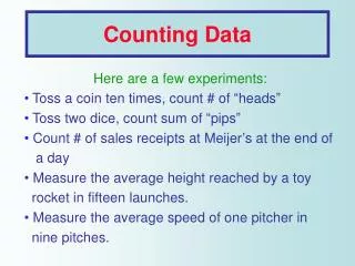
Counting Data Here are a few experiments: Toss a coin ten times, count # of “heads” Toss two dice, count sum of “pips” Count # of sales receipts at Meijer’s at the end of a day Measure the average height reached by a toy rocket in fifteen launches. Measure the average speed of one pitcher in nine pitches.
THE QUESTION: What do these separate experiments have in common? mmmm ……. Any takers?
THE ANSWER The end result is always A NUMBER !
RANDOM VARIABLES Quite clearly one cannot predict what number one gets from an experiment. That number therefore can be said to vary at random. We join the two concepts (variation and randomness) in a double term: Random Variable (RV for short) RVs can be thought of as functions that attach a number to each simple outcome of the experiment.
Types of RV’s • If all the possible values of a RV can be counted, we call that RV discrete. • Otherwise we say the RV is continuous. Let’s look at a few examples:
DiscreteorContinuous? • Sum of pips when tossing two dice DISCRETE • # of “Heads” in three coin tosses DISCRETE • # of coin tosses before the first “H” DISCRETE • The time it will take one of you to finish Thursday’s exam CONTINUOUS
Toss a coin ten times, count # of “heads” Discrete • Count # of sales receipts at Meijer’s at the end of a day Discrete • Measure the average height reached by a toy rocket in fifteen launches. Continuous • Measure the average speed of one pitcher in nine pitches. Continuous • Number of tosses of one die before a 6 shows up. Discrete
The Probability Distributionof a Random Variable Recall that RVs can be thought of as functions that attach a number to each simple outcome of the experiment. The collection of numbers that a RV can achieve is called the range of the RV. Let’s look at an example.
Toss two tetrahedra • Here is the sample space of tossing two tetrahedra and recording the sum of the two landed-on faces.
Let X be the RV “sum of the two faces.” Then the range of X clearly is {2, 3, 4, 5, 6, 7, 8} And P(2) = 1/16; P(3) = 2/16; P(4) = 3/16; P(5) = 4/16 ; P(6) = 3/16; P(7) = 2/16; P(8) = 1/16. We summarize the above with a table:
Another Example • Toss an unfair coin 4 times. The coin favors “H” 6 to 4, that is P(H)=0.6. • Let X = # of “Tails”. The range is clearly {0, 1, 2, 3, 4} We will learn later that So we get the probability distribution table:
Distribution Table: For discrete RVs a table or a formula generally suffice to describe the distribution, for continuous RV the situation will require graphs and a little geometry. We’ll do that later.
The Expected Value • Here is the Probability Distribution Table of a RV originating from some unspecified experiment Suppose you repeat the experiment 20 times.
Since “probability” really means “expected relative frequency” you would expect • 3 to happen 4 times (0.20x20) • 5 to happen 7 times (0.35x20) • 6 to happen 6 times (0.30x20) • 8 to happen 3 times (0.15x20) If you add up all these 20 numbers and then divide by 20 you get the mean (average) of the results. But this operation gives:
(follow closely) By the way, the answer is 5.35 We call this number the “expected value” of the random variable X and denote it by oror E(X) .
Formal Definition • Following the pattern suggested by the previous example we give the definition: Let be the probability distribution table of a random variable X. The expected value of X, denoted by = E(X), is the number
Final Remarks Remark # 1. Remember that Remark # 2. If in the equation all numbers but one are known, the unknown can be computed.
The Advantages of RV’s • For a mathematician or a statistician the most important benefit from using RVs is that: 1. Even though they are just probability spaces, the simple outcomes are justNUMBERS, not coins or dice or babies or patients. This leads us to the second advantage 2. Totally different real life situations may give rise to RVs with identical or at least
similar probability distributions. Here is an example of four separate situations that end up with identical RVs. • An unfair coin favors Heads 7 to 3. Toss it five times, count Heads. • A bag has 70 quarters and 30 dimes. Pick one coin from the bag, record its monetary value, put it back in the bag. Do this five times and add up the amounts you got. • 30% of the daily visitors to the Sporcizia Clinic develop a bacterial infection. Five patients came in today. Count how many did not develop the infection. • 30% of the students at Podunk U. cheat a little. Of five students chosen at random, count the honest ones.
Note that the events Heads, Quarters, No Infection, Honest are events with the same probability 0.7, and in all four of the examples we are counting how many times the event happens in five attempts. This leads to theprobability distribution table: where We will learn later that the pk ‘s add up to 1.
Another example • Nature favors girls 52 to 48. A couple decides to keep having babies until a boy is born or they have six girls, whichever happens first (in my hometown there was a family of 12 girls and one boy, spoiled rotten he ended up in jail). X is the number of children in that family. • A lot of 1,000 teething rings made in Lower Slobbovia is known to have 520 with excessive lead concentration. You keep buying a teething ring until you get a good one or you have bought six. X counts how many rings you buy.
In both examples you end up with a RV X whose probability distribution table is: Where We will learn later that the pk‘s add up to 1.
Special RVs The lesson to be garnered from the previous examples is that a particular probability distribution table can cover a multitude of seemingly different real life situations. So it behooves us to study individual RVs, each with its own model of a Probability Distribution Table. We say we are studying Random Variables, but we are really studying Distributions! What identifies a distribution ?
The distribution tables we have seen so far all look like this: To fill the table we need to know: 1. The top row 2. The bottom row This boils down to 1. The range of values 2. The individual probabilities
Special RV’s (cont’d) Let’s start easy. Here is a probability distribution table, let’s fill it: The top is any number The bottom must be 100% (This RV is neither R nor V, it’s called a constant)
A little harder: The top is any two numbers(usually 1 and 0) The bottom is any two p and q, both non negative, with p + q = 1 This RV has a name, Bernoulli RV, we look at when it happens.
Bernoulli Trials The Bernoulli RV happens whenever the experiment has just two possible numerical outcomes. In fact, if the actual outcomes are not numerical we can make them so by calling one of them 1 and the other 0 (we could also use 17 or 347, but it gets cumbersome!) In everyday practice the two outcomes are called “success” (corresponding to 1) and “failure” (corresponding to 0). Careful …
The two words “success” and “failure” do not have to maintain their usual meaning, in some experiment success may mean the fish died, or the rocket exploded, or the baby was a female(I am being sexist, just for fun!) In our context, success simply means the outcome that corresponds to the value 1, and failure means the outcome corresponding to the value 0.