Download
1 / 98
980 likes | 1.01k Views
Learn about well-separated pair decomposition (WSPD) and how it can be used to find t-spanners, approximate minimum spanning trees, and more in point sets. This lecture covers the construction algorithm for WSPD using compressed quadtrees.

E N D
Overview • Well Separated Pair Decomposition (WSPD) of a set of points, and how to find it. • Applications: • Finding a t-spanner of a set of points. • Approximating a minimum spanning trees of a point set. • Approximating the diameter of a point set. • Finding the closest pair. • All nearest neighbors problem. • Semi-separated pair decomposition.
Motivation • Let P be a set of n points in , we can represent all distances between points of P by explicitly listing the pairwise distances. • Moreover, the listing of coordinates of each point costs of memory. • We are interested in an alternative representation that will capture the structure of the distances between points.
Example • We would like to have a representation that captures the fact that p has similar distance to q and r, and furthermore, that q and r are close together as p is concerned. • If we are interested in the closest pair among the three points, we will only check q and r.
Definition 3.1 • The pair of the sets A and B is the set : The set of all the (unordered) pairs of points formed by the sets A and B. • We are interested in schemes that cover all possible pairs of points of P by small collection of such pairs.
Definition 3.1 [Pair Decomposition] • For a point set P , a pair decomposition of P is a set of pairs such that : • for every • for every • Translation : For any pair of distinct points there is at least one (and usually exactly one) pair such that and .
Example [Pair Decomposition] a d b c
Definition 3.2 • The pair Q and R is - separated if: Where : • In other words, imagine covering the two point sets with two balls of minimum size, and require that the distance between the two balls is at least the radius of the larger of the two.
Example [Well Separated Pair] B d(A,B) diam(B) A diam(A)
Definition 3.3 [WSPD] • For a point set P , a well-separated pair decomposition (WSPD) of P with parameter is a pair decomposition of P with a set of pairs : such that , for any i, the sets and are - separated.
Corollary 3.4 • For an - WSPD , it holds, for any pair ,that
Example of WSPD • Here is an example of - WSPD of a set of points P: A point set The decomposition into pairs The ½ WSPD
Reminder – Quadtrees(1) • Before seeing the constructing algorithm of WSPD, we will recall the quadtree data structure. • Given a set of points, we partition a square region containing the points to 4 equal-sized squares by horizontal and vertical cuts, and keep doing it recursively on each square until the square is empty or there is only 1 point inside it.
Reminder – Quadtrees(2) • In a quadtree : • Each node v corresponds to a cell . • The root node corresponds to the unit square. • Each node has 4 children, representing 4-equal sized squares inside it. • The leaves are the points.
Reminder – Quadtrees(3) • Compressed Quadtree: • Quadtrees may contain a lot of “useless” nodes , we can replace a sequence of useless edges by a single edge. • We will store inside each quadtree node v its square , and its level . • A compressed quadtree has a linear size. • There is an efficient construction of a compressed quadtree given a set of n points in time.
Reminder – Quadtrees(4) Examples of compressed and un-compressed quadtrees :
The algWSPD algorithm • We define as the diameter of the cell associated with the node v of the quadtree, but, if v contains a single point or is empty, we define . • , ) =
The construction algorithm for WSPD • Given a point set P in , the algorithm first computes the compressed quadtree T of P in . Next it computes the WSPD by calling , where is the root of T.
Example[1] u e v d f w a b c
Example[2] Assume
Example[3] Assume
Example[4] Assume
Example [6] • The returned set will be : • Definition - For a quadtree cell u :
Lemma 3.5 • Let □ be a cell of a grid G of with a cell diameter x. For , the number of cells in G at distance at most y from □ is . Proof : on board.
Lemma 3.6 • algWSPD terminates and computes a valid pair decomposition. • Proof: • By induction, it follows that every pair of points of P is covered by a pair of subsets output by algWSPD. • algWSPD always stops if both u and v are leaves, which implies that algWSPD always terminates. • Observe that if is in the output pair and either is not a single point, then , this implies that . Namely, . ▨
Lemma 3.7 • For the WSPD generated by algWSPD , we have that for any pair in the WSPD: For any • Proof: For every output pair we have by the design of the algorithm that : Also, for any , we have since and ▨
Lemma 3.8 (1) • For any pair , computed by algWSPD, we have that : where denotes the parent node x in the tree T.
Lemma 3.8 (2) • Proof : We trivially have that and . • A pair is generated because of a sequence of recursive calls where and is the root of T.
Lemma 3.8 (3) • Assume that • then since the algorithm always refines the larger cell. • Similarly, let t be the last index such that . Then, since v is a descendant of it hold that ▨
Lemma 3.9 • The number of pairs in the computed WSPD is .
Proof of lemma 3.9(1) • Let {u,v} be a pair appearing in the output. Consider the sequence of recursive calls that led to this output. Assume that the last recursive call to algWSPD(u,v) was issued by algWSPD(u,v’). Where is the parent of v in T. then by lemma 3.8. • Since the pair {u,v’} was not output by algWSPD, we conclude that and as such .
Proof of lemma 3.9(2) • Now, there are several possibilities: • : There are at most nodes that have the same level (i.e. diameter) as v’ such that their cells are within a distance at most r from it, by lemma 3.5. Thus, this type of charge can happen at most times, since v’ has at most children.
Proof of lemma 3.9 (3) • 2. : by the same argumentation, . There are at most such nodes . Since node has at most children, it follows that the number of such charges is at most .
Proof of lemma 3.9(4) • 3. : Consider the grid G having as one of its cells. Let be the cell in G containing . Observe that . In addition, . It follows that there are at most cells like that might participate in charging v’, and as such, the total number of charges is , as claimed.
Proof of lemma 3.9 (5) • v’ can be charged at most times. • This implies that the total number of pairs generated by the algorithm is , since the number of nodes in T is . ▨
Theorem 3.10 • For , one can construct an - WSPD of size , and the construction time is . • Proof: the running time of algWSPD is linear in the output size which is .
Applications of WSPD • Calculating a t-spanner of a set of points • Approximating the minimum spanning tree of a graph. • Approximating the diameter of a point set • Finding the closest pair • All nearest neighbors problem
Spanners – Definition 3.11 • For a weighted graph G and any two vertices q and s of G, we will denote by the graph distance between q and s. Formally, is the length of the shortest path in G between q and s. • Naturally, if q and s belongs to two different connected components of G, then .
Definition : t-spanner • A t-spanner of a set of points is a weighted graph G whose vertices are the points of P , and for any , we have : • The ratio is the stretch of q and s in G. • The stretch of G is the maximum stretch of any pair of points of P. • A t-spanner is a connected graph.
Example of a 3-spanner A B 5 (1,0) (2,3) 2 100 (-5,4) (0,0) 10 D C For example:
Theorem 3.12 • Given a set P of n points in and a parameter , one can compute a -spanner of P with edges in time. • Proof: First we will see the construction algorithm.
A construction algorithm of t-spanner • Let be an arbitrary constant, and set . Compute a - WSPD of P using algWSPD. • For any vertex u in the quadtree T of P (used in computing the WSPD), let be an arbitrary point of . For every pair , add an edge between with weight , and let G be the resulting graph.
Correctness proof (1) • We will prove that the returned graph is a -spanner of P. • By induction on the size of sets in WSPD we can prove that G is a connected graph and contains all point of P. • Observe that by the triangle inequality, we have that for any .
Correctness proof (2) • The upper bound on the stretch is proved by induction on the distance between 2 points in p. • So, fix a pair , and assume that by the induction hypothesis, for any pair such that , it follows that . • The pair x,y must appear in some pair , where .
Correctness proof (3) • Thus, by construction: , and this implies: . v u y x
Correctness proof (4) • Now, we can apply the induction hypothesis (twice) to the pairs of points and , implying that: and v u y x
Correctness proof (3) • Now, since is an edge of G, . • Thus, by the inductive hypothesis, the triangle inequality and (3.1), we have that : • (triangle inequality) (by the inductive hypothesis) And we proved the upper bound.▨ • The last step follows by an easy calculation, since , we have that: