Download
1 / 27
270 likes | 346 Views
Exploring Data. Edward Son and Michael Kim. Categorical Pie Bar Graph Quantitative Stem Plot Histogram Time Plot Ogive. Pie Charts. - Must include all the categories that make up a whole - Use When you want to emphasize each category’s relation to the whole. . Bar Graph .

E N D
Exploring Data Edward Son and Michael Kim
Categorical • Pie • Bar Graph • Quantitative • Stem Plot • Histogram • Time Plot • Ogive
Pie Charts - Must include all the categories that make up a whole - Use When you want to emphasize each category’s relation to the whole.
Bar Graph • Easy to make, easy to read • More flexible than pie charts • A graph drawn using rectangular bars to show how large each value is.
Stem Plot • Gives quick picture of the shape of a distribution while including actual numerical values • Making a stem plot - Separate each observation into a stem, consisting of all but the final digit, and a leaf, the final digit. - Write the stems in a vertical column with the smallest at the top, and draw a vertical line at the right of this column - Write each leaf in the row to the right of its stem, in increasing order out from the stem. Side-By-Side Stem Plot
Side-By-Side Stem Plot • Can double the number of stems in a plot by splitting stems into two • Can trim the numbers by removing the last digit or digits before making a stem plot is often the best
Histogram • Breaks the range of values of a variable into classes and displays only the count or percent of the observations that fall into each classes
Time Plot • A time plot of a variable plots each observation against the time at which it was measured. Always put time on the horizontal scale of your plot and the variable you are measuring on the vertical scale. • Displays of distribution that includes time.
Relative Frequency and Cumulative Frequency • Ogive Graph
Histograms vs Bar Graphs • Shows counts or percents of a quantitative variable. • Bars are connected • Displays categorical variable. • Bars are separated
Examining a Distribution • Use SOCS • S – Shape • O – Outlier • C – Center • S - Spread
Mode • S – Shape • Mode = Peaks (One major peak called Unimodal) • Skewedness • Symmetric Skewed right Symmetric
O- Outliers • An important kind of deviation is an outlier, an individual value that falls outside the overall pattern Outliers Outliers
C – Center • Describe the center of a distribution by its midpoint • Ex) mean, median (more information later)
S – Spread • Can describe by giving the smallest and largest values
Five Number Summary • Minimum • Q1 • Median • Q3 • Maximum
Quartiles • First Quartile Q1 • Third Quartile Q3 • Interquartile Range = Q3 – Q1
1.5 x IQR Rule • Use 1.5 x IQR Rule for suspected Outliers
Median • It is the midpoint of a distribution 1 1 4 1 2 7 3 10 4 1 5 6 6 7 7 7 3 7 7 8 9 4 2 1 1 1 2 2 3 4 4 4 5 6 6 7 7 7 7 7 7 8 9 10 3 Median
Mean • To find the mean of observations, add their values and divide by the number of observations x
Standard Deviation • The variance s^2 of a set of observations is the average of the squares of the deviations of the observations from their mean.
Shape: Slightly skewed left with on peak (unimodal). • Outliers: 1.5 x IQR so 1.5 x17=25.5 - Q1= 35-1.5 x 25.5 = -3.25 - Q3= 54+1.5 x 25.5 = 92.75 There fore there are no outliers. • Center: Approximately at 43.93 • Spread: Babe Ruth’s number of home runs in a single season varies from a low of 23 to a high of 60.
Insert data in L1 in stat edit • Calculate 1 var stat or do it all in hand • Mean = 23.176 • Standard deviation = 18.639 • Median = 22
median Q3 Q1 Minimum value Maximum value
81 – 11 = 70 (45+47)/2 = 26