Panel E Linking HSM to population modeling

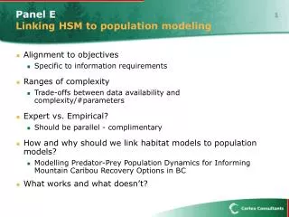
1. Panel ELinking HSM to population modeling • Alignment to objectives • Specific to information requirements • Ranges of complexity • Trade-offs between data availability and complexity/#parameters • Expert vs. Empirical? • Should be parallel - complimentary • How and why should we link habitat models to population models? • Modelling Predator-Prey Population Dynamics for Informing Mountain Caribou Recovery Options in BC • What works and what doesn’t?

2. Spatial Output from MC-HSM Potential Potential Potential Potential Potential Potential Potential Potential Potential Potential Potential Potential Predator Predator Predator Predator Predator Predator Potential Potential Potential Potential Potential Potential Predator Predator Predator Predator Predator Predator Prey Potential Density Density Density Density Density Density Density Predator Predator Predator Predator Predator Predator Background Predation Predator Efficiency Road Density Road Density Road Density Density Density Density Density Density Density Time Series Time Series Time Series Density Density Density Density Density Density Potential Potential Potential Potential Potential Potential Predator Predator Predator Potential Potential Potential Predator Predator Predator Density Density Density Predator Predator Predator Road Density Road Density Road Density Density Density Density Time Series Time Series Time Series Density Density Density Spatial Preprocessing Walter’s Multi-Species Disc Equation Population Structure Ungulates Mortality & Recruitment Predators Rate of Increase Mortality Rates Population Dynamics Output Indicators Conceptual Model Model Outputs Disc Equation Parameters 1) Rate of Effective Search (ai) • search rate (km2/day) X prob kill given encounter • modified by predator search rate adjustment factor 2) Time spent in strata (Ti) • sum of search time and handling time • estimated based on potential edible biomass for strata 3) Prey density in strata (Ni) 4) Handling time for prey (hj)

3. Model Development Spatial Aspects of Model • Preprocessing Step • For each prey species and each season • Expected Value for potential density, PSRA, and CAM is drawn from mean and sd for each 1ha cell

4. Model Development Spatial Aspects of Model • Preprocessing Step • For each prey species and each season • Expected Value for potential density, PSRA, and CAM is drawn from mean and sd for each 1ha cell • Layers rescaled from 100x100m to 1000 x1000m, using mean

5. Model Development Spatial Aspects of Model • Prey population is distributed in each cell based on the relative densities Expected Potential Density (i.e., expected values from BBN)

6. Model Development Spatial Aspects of Model • Prey population is distributed in each cell based on the relative densities Matrix sums to one Relative Densityij= Expected Densityij/ ∑(Expected Densityij)

7. Model Development Spatial Aspects of Model • Expected density – integrated over the season Matrix sums to initial population size (e.g., 500) Expected Population Densityij = N * Relative Densityij

8. What works and what doesn’t? • Spatial models are CPU intensive • Uncertainty in parameter estimates -> stochastic model -> Multiple iterations • Decoupling spatial processing from a spatial population model