Particle Systems

Particle Systems CSE169: Computer Animation Instructor: Steve Rotenberg UCSD, Winter 2004

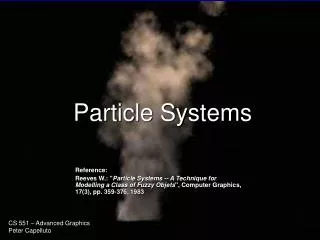
Particle Systems • Particle systems have been used extensively in computer animation and special effects since their introduction to the industry in the early 1980’s • The rules governing the behavior of an individual particle can be relatively simple, and the complexity comes from having lots of particles • Usually, particles will follow some combination of physical and non-physical rules, depending on the exact situation

Physics

Kinematics of Particles • We will define an individual particle’s 3D position over time as r(t) • By definition, the velocity is the first derivative of position, and acceleration is the second

Kinematics of Particles • To render a particle, we need to know it’s position r.

Uniform Acceleration • How does a particle move when subjected to a constant acceleration?

Uniform Acceleration • This shows us that the particle’s motion will follow a parabola • Keep in mind, that this is a 3D vector equation, and that there is potentially a parabolic equation in each dimension. Together, they form a 2D parabola oriented in 3D space • We also see that we need two additional vectors r0 and v0 in order to fully specify the equation. These represent the initial position and velocity at time t=0

Mass and Momentum • We can associate a mass m with each particle. We will assume that the mass is constant • We will also define a vector quantity called momentum (p), which is the product of mass and velocity

Newton’s First Law • Newton’s First Law states that a body in motion will remain in motion and a body at rest will remain at rest- unless acted upon by some force • This implies that a free particle moving out in space will just travel in a straight line

Force • Force is defined as the rate of change of momentum • We can expand this out:

Newton’s Second Law • Newton’s Second Law says: • This relates the kinematic quantity of acceleration to the physical quantity of force

Newton’s Third Law • Newton’s Third Law says that any force that body A applies to body B will be met by an equal and opposite force from B to A • Put another way: every action has an equal and opposite reaction • This is very important when combined with the second law, as the two together imply the conservation of momentum

Conservation of Momentum • Any gain of momentum by a particle must be met by an equal and opposite loss of momentum by another particle. Therefore, the total momentum in a closed system will remain constant • We will not always explicitly obey this law, but we will implicitly obey it • In other words, we may occasionally apply forces without strictly applying an equal and opposite force to anything, but we will justify it when we do

Energy • The quantity of ‘energy’ is very important throughout physics, and the motion of particle can also be formulated in terms of energy • Energy is another important quantity that is conserved in real physical interactions • However, we will mostly use the simple Newtonian formulations using momentum • Occasionally, we will discuss the concept of energy, but probably won’t get into too much detail just yet

Forces on a Particle • Usually, a particle will be subjected to several simultaneous vector forces from different sources • All of these forces simply add up to a single total force acting on the particle

Particle Simulation • Basic kinematics allows us to relate a particle’s acceleration to it’s resulting motion • Newton’s laws allow us to relate acceleration to force, which is important because force is conserved in a system and makes a useful quantity for describing interactions • This gives us a general scheme for simulating particles (and more complex things):

Particle Simulation 1. Compute all forces acting within the system (making sure to obey Newton’s third law) 2. Compute the resulting acceleration for each particle (a=f/m) and integrate to get positions - Repeat • This describes the standard ‘Newtonian’ approach to simulation. It can be extended to rigid bodies, deformable bodies, fluids, vehicles, and more

Particle Example class Particle { float Mass; // Constant Vector3 Position; // Evolves frame to frame Vector3 Velocity; // Evolves frame to frame Vector3 Force; // Reset and re-computed each frame public: void Update(); void Draw(); void ApplyForce(Vector3 &f) {Force.Add(f);} };

Particle Example class ParticleSystem { int NumParticles; Particle *P; public: void Update(); void Draw(); };

Particle Example ParticleSystem::Update(float time) { // Compute forces Vector3 gravity(0,-9.8,0); for(i=0;i<NumParticles;i++) { Vector3 force=gravity*Particle[i].Mass; // f=mg Particle[i].ApplyForce(force); } // Integrate for(i=0;i<NumParticles;i++) Particle[i].Update(time); }

Particle Example Particle::Update(float time) { // Compute acceleration (Newton’s second law) Vector3 Accel=(1.0/Mass) * Force; // Compute new position & velocity Velocity+=Accel*time; Position+=Velocity*time; // Zero out Force vector Force.Zero(); }

Particle Example • With this particle system, each particle keeps track of the total force being applied to it • This value can accumulate from various sources, both internal and external to the particle system • The example just used a simple gravity force, but it could easily be extended to have all kinds of other possible forces • The integration scheme used is called ‘forward Euler integration’ and is about the simplest method possible

Forces

Uniform Gravity • A very simple, useful force is the uniform gravity field: • It assumes that we are near the surface of a planet with a huge enough mass that we can treat it as infinite • As we don’t apply any equal and opposite forces to anything, it appears that we are breaking Newton’s third law, however we can assume that we are exchanging forces with the infinite mass, but having no relevant affect on it

Gravity • If we are far away enough from the objects such that the inverse square law of gravity is noticeable, we can use Newton’s Law of Gravitation:

Gravity • The law describes an equal and opposite force exchanged between two bodies, where the force is proportional to the product of the two masses and inversely proportional to their distance. The force acts in a direction e along a line from one particle to the other (in an attractive direction)

Gravity • The equation describes the gravitational force between two particles • To compute the forces in a large system of particles, every pair must be considered • This gives us an N2 loop over the particles • Actually, there are some tricks to speed this up, but we won’t look at those

Aerodynamic Drag • Aerodynamic interactions are actually very complex and difficult to model accurately • A reasonable simplification it to describe the total aerodynamic drag force on an object using: • Where ρ is the density of the air (or water…), cd is the coefficient of drag for the object, a is the cross sectional area of the object, and e is a unit vector in the opposite direction of the velocity

Aerodynamic Drag • Like gravity, the aerodynamic drag force appears to violate Newton’s Third Law, as we are applying a force to a particle but no equal and opposite force to anything else • We can justify this by saying that the particle is actually applying a force onto the surrounding air, but we will assume that the resulting motion is just damped out by the viscosity of the air

Springs • A simple spring force can be described as: • Where k is a ‘spring constant’ describing the stiffness of the spring and x is a vector describing the displacement

Springs • In practice, it’s nice to define a spring as connecting two particles and having some rest length l where the force is 0 • This gives us:

Springs • As springs apply equal and opposite forces to two particles, they should obey conservation of momentum • As it happens, the springs will also conserve energy, as the kinetic energy of motion can be stored in the deformation energy of the spring and later restored • In practice, our simple implementation of the particle system will guarantee conservation of momentum, due to the way we formulated it • It will not, however guarantee the conservation of energy, and in practice, we might see a gradual increase or decrease in system energy over time • A gradual decrease of energy implies that the system damps out and might eventually come to rest. A gradual increase, however, it not so nice… (more on this later)

Dampers • We can also use damping forces between particles: • Dampers will oppose any difference in velocity between particles • The damping forces are equal and opposite, so they conserve momentum, but they will remove energy from the system • In real dampers, kinetic energy of motion is converted into complex fluid motion within the damper and then diffused into random molecular motion causing an increase in temperature. The kinetic energy is effectively lost.

Dampers • Dampers operate in very much the same way as springs, and in fact, they are usually combined into a single spring-damper object • A simple spring-damper might look like: class SpringDamper { float SpringConstant,DampingFactor; float RestLength; Particle *P1,*P2; public: void ComputeForce(); };

Dampers • To compute the damping force, we need to know the closing velocity of the two particles, or the speed at which they are approaching each other • This gives us the instantaneous closing velocity of the two particles

Dampers • Another way we could compute the closing velocity is to compare the distance between the two particles to their distance from last frame • The difference is that this is a numerical computation of the approximate derivative, while the first approach was an exact analytical computation

Dampers • The analytical approach is better for several reasons: • Doesn’t require any extra storage • Easier to ‘start’ the simulation (doesn’t need any data from last frame) • Gives an exact result instead of an approximation • This issue will show up periodically in physics simulation, but it’s not always as clear cut

Force Fields • We can also define any arbitrary force field that we want. For example, we might choose a force field where the force is some function of the position within the field • We can also do things like defining the velocity of the air by some similar field equation and then using the aerodynamic drag force to compute a final force • Using this approach, one can define useful turbulence fields, vortices, and other flow patterns

Collisions & Impulse • A collision is assumed to be instantaneous • However, for a force to change an object’s momentum, it must operate over some time interval • Therefore, we can’t use actual forces to do collisions • Instead, we introduce the concept of an impulse, which can be though of as a large force acting over a small time

Impulse • An impulse can be thought of as the integral of a force over some time range, which results in a finite change in momentum: • An impulse behaves a lot like a force, except instead of affecting an object’s acceleration, it directly affects the velocity • Impulses also obey Newton’s Third Law, and so objects can exchange equal and opposite impulses • Also, like forces, we can compute a total impulse as the sum of several individual impulses

Impulse • The addition of impulses makes a slight modification to our particle simulation:

Collisions • Today, we will just consider the simple case of a particle colliding with a static object • The particle has a velocity of v before the collision and collides with the surface with a unit normal n • We want to find the collision impulse j applied to the particle during the collision

Elasticity • There are a lot of physical theories behind collisions • We will stick to some simplifications • We will define a quantity called elasticity that will range from 0 to 1, that describes the energy restored in the collision • An elasticity of 0 indicates that the closing velocity after the collision is 0 • An elasticity of 1 indicates that the closing velocity after the collision is the exact opposite of the closing velocity before the collision

Collisions • Let’s first consider a collision with no friction • The collision impulse will be perpendicular to the collision plane (i.e., along the normal) • That’s actually enough for collisions today. We will spend a whole lecture on them next week.

Combining Forces • All of the forces we’ve examined can be combined by simply adding their contributions • Remember that the total force on a particle is just the sum of all of the individual forces • Each frame, we compute all of the forces in the system at the current instant, based on instantaneous information (or numerical approximations if necessary) • We then integrate things forward by some finite time step

Integration

Integration • Computing positions and velocities from accelerations is just integration • If the accelerations are defined by very simple equations (like the uniform acceleration we looked at earlier), then we can compute an analytical integral and evaluate the exact position at any value of t • In practice, the forces will be complex and impossible to integrate analytically, which is why we automatically resort to a numerical scheme in practice • The Particle::Update() function described earlier computes one iteration of the numerical integration. In particular, it uses the ‘forward Euler’ scheme

Forward Euler Integration • Forward Euler integration is about the simplest possible way to do numerical integration • It works by treating the linear slope of the derivative at a particular value as an approximation to the function at some nearby value • The gradient descent algorithm we used for inverse kinematics used Euler integration

Forward Euler Integration • For particles, we are actually integrating twice to get the position which expands to

Forward Euler Integration • Note that this: is very similar to the result we would get if we just assumed that the particle is under a uniform acceleration for the duration of one frame:

Particle Systems