Download
1 / 74
780 likes | 1.09k Views
Measuring Interest Rate Risk. Judson W. Russell, Ph.D., CFA. CONFIDENTIAL. DRAFT. Module 1: Economy & Sovereign Risk. Debt to Nominal GDP. Recession – Part 2?. Sovereign Risk - Portugal. 5. Sovereign Risk - France. 6. Sovereign Risk - Spain. 7. A Good Place to Be This Year?. 8.

E N D
Measuring Interest Rate Risk Judson W. Russell, Ph.D., CFA CONFIDENTIAL DRAFT
Fair Value Framework 10 Year Rate = f(Fed Funds target, short-term (1y) inflation expectations, long-term (10y), 1y expectation of real GDP growth, term premium) 10
Use Inflation Swap to Observe Inflation Expectations Zero Coupon Inflation Swap : Client Pays Fixed Rate 11
Term Premium • The term spread—the observed difference between the yield on a long-term and a short-term bond—reflects a combination of underlying factors. • Its largest component is investors’ expectations about future short-term interest rates. We refer to • the difference between average expected short-term rates over the lives of the two bonds as the expectations component of the term spread. • The remaining difference in yield compensates investors for the risks associated with holding long-term rather than short-term investments. We call this the term premium component. Neither component is directly observable, so we measure term premia using a statistical model (Kim-Wright) and attribute the balance of the term spread to the expectations component. • The relationship between the term spread and its components is given in equation 1: • term spread = expectations component + term premium component. • In turn, each component includes both inflation-related and real factors: • (2) expectations component = inflation expectations + real rate expectations • (3) term premium component = inflation risk premium + real rate risk premium. • Changes in the term premium component are expected to be driven primarily by the long-term risk outlook, since relatively little compensation is needed for short-term risk. We would thus expect the term premium component to decline as investor uncertainty about long-term productivity improves (indicating reduced real rate risk) and as inflation expectations become more stable. 12
Concept Check 1a With the yield curve historically steep (2s5s at 74bp), how can this be called an inversion? 13
Concept Check 1a - Answer With the yield curve historically steep (2s5s at 74bp), how can this be called an inversion? With front-end rates near zero, there is a limit on potential decline. The long position in a forward rate is implicitly short a floor struck at zero. Usually this option can be ignored, but no longer the case. The 4yfwd1y Treasury has declined to historical lows since July, but implied vol on 4y1y swaption has only modestly declined. 4y1y vol of 102 bp implies 204bp for one std deviation of the 1y rate over a 4-year time period. Close to the 2.1% level on 4yfwd1y rate. 14
Concept Check 1b A Rates Strategist is currently recommended 10s-30s flatteners to clients. What does this mean and what is her view? 15
Concept Check 1b - Answer A Rates Strategist is currently recommended 10s-30s flatteners to clients. What does this mean and what is her view? A Flattener is a bet that the yield curve will flatten. Sell the short end, and buy the long end. Duration weight the trade to hedge parallel-shifts in the curve. Given the Fed’s Twist program there is a negative net supply to the long bond. The strategist suggests that there could be an additional 35 bp from current levels. 16
Interest Rate Risk Management Berkshire Hathaway showed a pretax gain of $1.5 billion from selling U.S. government bonds during 2003. “The profits in governments arose from our liquidation of long-term strips (the most volatile of government securities).” Warren Buffett from Berkshire Hathaway Annual Report 2003. 18
Price Volatility • Two approaches to measure the price volatility of bonds due to movements in the interest rates are: • full valuation approach • duration/convexity approach Do you notice a pattern in the price change for a given change in yield? 19
Properties of Bond Price Volatility • For very small changes in yield the magnitude of the percentage price change for different bonds is about equal, whether the yield increases or decreases. • For large changes in yield, the magnitude of the percentage price change depends on whether the yield increases or decreases. Notice the larger price increase as yields fall relative to when they rise. 20
Properties of Bond Price Volatility • The percentage price change on a bond for a given change in interest rates depends on three key features: 1. Coupon rate • all else equal, the lower the coupon, the greater the bond price volatility 2. Term to maturity • the longer the term to maturity, the greater the bond price volatility 3. Initial yield • the lower the initial yield, the greater the price volatility 21
Challenge Problem - Answer 1. Coupon rate: all else equal, the lower the coupon, the greater the bond price volatility 2. Term to maturity: the longer the term to maturity, the greater the bond price volatility 3. Initial yield: the lower the initial yield, the greater the price volatility Therefore, A is true due to 2., C is true due to 1., D is true—B is false. Duration is greater with lower yield to maturity. 23
Full Valuation Approach • The full valuation approach simply applies the basic bond valuation equations using hypothetical yield changes. • Begin with the current market yield and price • Estimate the hypothetical changes in required yields • Re-compute bond prices using the new required yields • Compare the resulting price changes 24
Full Valuation Approach • We will look at the full valuation approach using two bonds and a portfolio when there are parallel shifts in the yield curve, of +50 bps and +100 bps. • You have a $10 million face-value position in both X and Y. 25
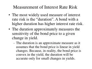
Duration • Duration is the most widely used measure of bond price volatility. • This measure captures the impact of coupon, maturity, and initial yield in one number. • Formally, duration is the first derivative of the bond’s price function with respect to yield. • Duration is a measure of a bond’s (or portfolio’s) sensitivity to a 1% change in interest rates. 26
Duration • “In managing the Portfolio, we seek to maintain an effective duration of one to three years under normal market conditions.” AllianceBernstein Short Duration Portfolio • “Based on our long-term, fundamental outlook for the economy and interest rates, we set our portfolio duration in a range that is typically plus or minus 10 percent of the benchmark duration. Key factors in determining portfolio duration are inflation rates, fiscal policy, monetary policy, and the business cycle.” Advantus Capital Full Duration Fixed Income Principal Global High Quality Core Fixed Income Fund 27
Duration • Macaulay’s duration • Developed by Frederick Macaulay in 1938. • Discounted time-weighted cash flow of the security divided by the price • Consider a 4-year annual pay, 8% coupon bond priced to yield 8% $1,000 = 80/(1.08)1 + 80/(1.08)2 + 80/(1.08)3 + 1,080/*(1.08)4 $1,000 = 74.074 + 68.587 + 63.507 + 793.832 Discounted time-weighted cash flow: 74.074 (1) + 68.587 (2) + 63.507 (3) + 793.832 (4) = 3,577.097 Divided by price = 3.577 years 28
Duration • Macaulay’s duration • Fulcrum in the timeline of security’s life where the reinvested cash flows exactly balance out the present value of the remaining future cash flows. What is the Macaulay’s duration for a four-year, zero coupon bond? 80 80 80 1,080 0 1 2 3 3.577 4 29
Duration • Macaulay’s duration (4-year, 8% coupon annual pay, yielding 8%) 30
Duration • Macaulay’s duration (4-year, zero coupon annual compounding 8%) 31
Duration • Macaulay’s duration (4-year, zero coupon annual compounding 12%) 32
Duration • Modified duration is derived by making a small modification to the Macaulay duration value. • To obtain the modified duration, we simply divide the Macaulay duration value by 1 plus the current yield to maturity divided by the number of payments in a year. DMAC = 3.577 DMOD = 3.577/(1+0.08/1) = 3.312 • Modified duration provides an approximation to the interest rate sensitivity of a bond. 33
Modified Duration • Suppose you manage the portfolio that we used in the earlier example (bonds X and Y). • Duration for Bond X (5-year, annual pay 8% coupon, yielding 6%) 35
Modified Duration • Duration for Bond Y (15-year, annual pay 5% coupon, yielding 7%) 36
Modified Duration • With $10 million invested in each bond, your portfolio duration is simply the weighted average of duration for the components of the portfolio: (1/2) DMOD,Bond X + (1/2) DMOD,Bond Y = D MOD, Portfolio (1/2) 4.10 + (1/2) 9.73 = 6.92 • This implies that if interest rates increased by 100 bps, your portfolio would lose 692 bps (6.92%). • Using the full valuation approach we saw that the true change was 620 basis points. 37
Modified Duration • Earlier we stated that changes were fairly consistent for small changes in yield, but differed for large changes in yield. • Duration is a good approximation for small changes in yield, but is not sufficient for large changes in yield. 38
Challenge Problem - Answer D is incorrect 40
Effective Duration • We saw that changes in bond price for changes in yield were influenced by the initial location on the price-yield graph. 41
Effective Duration • We can capture the effective duration using the following formula: Effective duration = [(V- -V+) / (2V0(Dy))] where: V- = estimated price if yield decreases by a given amount, Dy V+ = estimated price if yield increases by a given amount, Dy V0 = initial observed bond price Dy = change in required yield, in decimal form 42
Effective Duration Example • Suppose there is a 5-year, semi-annual pay, option free non-callable bond with an annual coupon of 7.25% trading at 98. If interest rates rise by 50 basis points (0.50%), the estimated price of the bond is 96.01. If interest rates fall by 50 basis points, the estimated price of the bond is 100.04. The effective duration is: Effective duration = [(V- -V+) / 2V0(Dy)] Effective duration = [(100.04 - 96.01)/(2 x 98 x 0.005)] Effective duration = 4.11 43
Duration Effect • The duration effect shows how the price of the bond will respond to a specific change in yield. Duration Effect = -Duration x (Dy) Duration Effect = -4.11 x 0.005 Duration Effect = -2.055% Approximate price for a 50 bps increase in yield: 98 x (1-.02055) = 95.99. Actual price change for a 50 bps increase in yield = 96.01. 44
Challenge Problem Effective duration = [(V- -V+) / 2V0(Dy)] Effective duration = [(111.0 – 105.3)/(2 x 108.1 x 0.005)] Effective duration = 5.27 46
Effective vs Modified • Suppose there is a 5-year, semi-annual pay, bond callable at 102 with an annual coupon of 7.25% trading at 101. If interest rates rise by 50 basis points (0.50%), the estimated price of the bond is 98.935. If interest rates fall by 50 basis points, the bond is called at 102. The effective duration is: Effective duration = [(V- -V+) / 2V0(Dy)] Effective duration = [(102 - 98.935)/(2 x 101 x 0.005)] Effective duration = 3.03 47
Challenge Problem - Answer Effective duration = [(V- -V+) / 2V0(Dy)] Effective duration = [(105.56 – 98.46)/(2 x 101.76 x 0.01)] Effective duration = 3.49 49
Key Rate Duration • Holding all other maturities constant, this measures the sensitivity of a security or the value of a portfolio to a 1% change in yield for a given maturity.The calculation is as follows:Where:P- = Security's price after a 1% decrease in yield P+ = Security's price after a 1% increase in yield P0 = Security's original price • There are 11 maturities along the Treasury spot rate curve, and a key rate duration is calculated for each. The sum of the key rate durations along a portfolio yield curve is equal to the effective duration of the portfolio. 50