Download
1 / 65
650 likes | 752 Views
Explore the latest findings from WMAP, including insights on inflation models, CMB polarization, and the cosmological power spectrum. Learn about the DM/DE composition, new measurements, diverse research teams, and critical instrument stability.

E N D
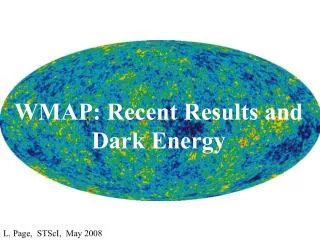
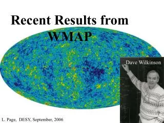
Recent Results from WMAP Dave Wilkinson L. Page, DESY, September, 2006
The Standard Cosmological Model Surface oflast scattering at “decoupling.” “Reionization”
The New Science Basic model agrees with virtually all cosmological measurements. The DM/DE composition is parametrized phenomenologically. Inflation-like models, based on field theories of the t<10-20s Universe, predict the gravitational landscape to which the contents respond, differ by 5% from the historic (PHZ) phenomenological description. WMAP observes this difference.
What’s New in the Measurement? Much better understanding of instrument, noise, gain, beams, and mapmaking. Direct measurement of CMB polarization at >100 angular scales. The error bars are near 300 nK. Three times as much data, smaller errors in maps: more than 50x reduction in model parameter space.
WMAP A partnership between NASA/GSFC and Princeton Science Team: NASA/GSFC Bob Hill Gary Hinshaw Al Kogut Michele Limon Nils Odegard Janet Weiland Ed Wollack Johns Hopkins Chuck Bennett (PI) UCLA Ned Wright Brown Greg Tucker Chicago Stephan Meyer Hiranya Peiris UBC Mark Halpern Princeton Norm Jarosik Lyman Page David Spergel. CITA Olivier Dore Mike Nolta Penn Licia Verde UT Austin Eiichiro Komatsu Cornell Rachel Bean Microsoft Chris Barnes
For temperature: measure difference in power from both sides. CMB: 30 uK rms (>100) For polarization: measure the difference between differential temperature measurements with opposite polarity. CMB 0.3 uK rms ) ( * * <ExEx> <ExEy> * * <EyEx> <EyEy> ( ( A-B-A-B B-A-B-A ) ) = I/2 0 + Q/2 U/2 One of 20 0 I/2 U/2 -Q/2 Amplifiers from NRAO, M. Pospieszalski design Intensity Stokes Q&U Coherency matrix
Stability of instrument is critical Physical temperature of B-side primary over three years. Model based on yr1 alone 3yr Model Three parameter fit to gain over three years leads to a clean separation of gain and offset drifts. Data based on dipole Jarosik et al.
Physical size = plasma speed X age of universe at decoupling Angular Power Spectrum. Power spectrum ~10 early in inflation ~0.40 later in inflation The overall tilt of this spectrum--- encoded in the “scalar spectral index” ns--- is the new handle on inflation.
CMB alone tells us we are on the “geometric degeneracy” line closed “Geometric Degeneracy” open { WMAP3 only best fit LCDM Assume flatness Reduced
Large Angular Scale Polarization The formation of the first stars produces free electrons that: (1) rescatter CMB photons thereby reducing the anisotropy and (2) polarize the CMB at large angular scales. These effects mimic a change in ns: “the ns - tau” degeneracy WMAP measures (2) to break the degeneracy
V Band, 61 GHz CMB 6 uK
From Wayne Hu CMB Polarization Polarization of the CMB is produced by Thompson scattering of a quadrupolar radiation pattern. E 2 deg Whenever there are free electrons, the CMB is polarized. B The polarization field is decomposed into “E” and “B” modes. Seljak & Zaldarriaga
Gravitational wave Density wave Terminology: E/B Modes k k E-modes B-modes
Types of Cosmological Perturbations Temperature Scalars: , E polarization Temperature Tensors: h (GW strain) E polarization B polarization 0.3 Or less! n and r are predicted by models of inflation.
Low-l EE/BB EE (solid) BB (dash) EE/BB model at 60 GHz r=0.3 Since reionization is late we see it at large angular scales. This is our handle on the optical depth.
Raw vs. CleanedMaps Galaxy masked in analysis
Low-l EE/BB EE BB BB Polarization: null check and limit on gravitational waves. EE Polarization: from reionization by the first stars r<2.2 (95% CL) from just EE/BB Just Q and V bands.
Degeneracy 1yr WMAP No SZ marg L WMAP1+ACBAR+CBI 3yr WMAP Knowledge of optical depth breaks the degeneracy
TT TE EE Approx EE/BB foreground BB inflation BB r=0.3 BB Lensing (not primordial)
Model needs , 8 Model needs not unity, 8 Model needs dark matter, 248 Model does not need: “running,” r, or massive neutrinos, < 3. What Does the Model Need to Describe the Data? changing one of the 6 parameters at a time…. { (“2.8 sigma”) ….but Eriksen & Huffenberger 0.959+/-0.016 WMAP 0.947+/-0.015 (all) (“15 sigma”) The data are, of course, less restrictive when there are more parameters.
Equation of State & Curvature Interpret as amazing consistency between data sets. WMAP+CMB+2dFGRS+SDSS+SN
Maps of Multipoles Too aligned? Too symmetric?
What’s Next? The CMB is still a scientific gold mine. Small scale anisotropy Polarization at all angular scales Better known parameters W not -1? Neutrino mass? Non-gaussanity? Something new? Non-adiabatic modes ? Formation and growth of cosmic structure. Tests of field theories at 10-35 s.
Selected Bolometer-Array and SZ Roadmap ACT (3000 bolometers) Chile BRAIN SCUBA2 SZA QUAD QUIET (12000 bolometers) (Interferometer) Owens Valley BiCEP CLOVER 2006 2007 2008 2005 SPT (1000 bolometers) South Pole Polarbear-I APEX (~400 bolometers) Chile (300 bolometers) California Planck (50 bolometers) L2
“large scale” (unique to satellite) 2 bumps R=0.01
ACT Science: Observations: CMB: l>1000 Growth of structure Eqn. of state Cluster (SZ, KSZ X-rays, & optical) Atacama Cosmology Telescope Neutrino mass Diffuse SZ Ionization history OV/KSZ Inflation Lensing Power spectrum X-ray Optical Theory Collaboration: Cardiff Columbia Haverford NIST CUNY Princeton INAOE NASA/GSFC Rutgers UBC UPenn U. Toronto U. Catolica U. KwaZulu-Natal UMass U. Pittsburgh
More simulations of mm-wave sky. Survey area High quality area 150 GHz SZ Simulation MBAC on ACT PLANCK Burwell/Seljak 1.5’ beam WMAP ACT Target Sensitivity (i.e. ideal stat noise only) PLANCK SPT & APEX as well. / Diffuse KSZ / Diffuse KSZ de Oliveira-Costa
Completed “close-packed” 12x32 bolometer array Torsional yoke attachment Linear array after folding Arrays of bolometers S. Staggs is lead Moseley et al, NASA/GSFC 3.2 mm Need picture SHARC II 12x32 Popup Array PI D. Dowell Irwin et al. SCUBA 1 mm Warm electronics based on SCUBA2 One element of array Halpern et al. UBC
Camera (MBAC) Layout 0.6K Pulse Tube 3He Fridge D. Swetz 40K Shield 3 feet AR Coated Si lenses. Filters: Cardiff
New Type of Telescope M. Devlin is lead Telescope at AMEC in Vancouver. Ship to Chile in 2006.
First Light Dec 05 CCAM Moon Measured from Jadwin Hall at 150 GHz with x11 attenuation. CCAM: A 1x32 muxed TES array prototype on the WMAP spare.
Foreground Model • Template fits (not model just shown). • Use all available information on polarization directions. • Sync: Based on K band directions • Dust: Based on directions from starlight polarization. • Increase errors in map for subtraction. • Examine power spectrum l by l and frequency. • Examine results with different bands. • Examine the results with different models. Band Pre-Cleaned Cleaned Table of Ka 2.14 1.096 Q 1.29 1.02 V 1.05 1.02 W 1.06 1.05 4534 DOF
High l TE Crittenden et al.
Frequency space “Spikes” from correlated polarized sync and dust.
Abbreviated The Standard Cosmological Model At a very early time a “quantum field” impressed on the universe a gravitational landscape. This is literally a picture of a quantum field from the birth of the universe. Matter fell into the valleys to form eventually “structure.” But only 1/6 of this matter is familiar to us. The dynamics of the universe is now driven not so much by the matter but by a new form of energy: “The Dark Energy.”
Compare Spectra First peak Cosmic variance limited to l=400. Window function dominates difference