Download
1 / 43
470 likes | 910 Views
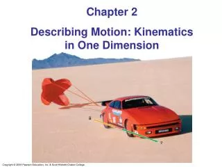
Ch. 2: Describing Motion: Kinematics in One Dimension. Terminology. Classical Mechanics = The study of objects in motion. 2 parts to mechanics. Kinematics = A description of HOW objects move. Chapters 2 & 4 (Ch. 3 is mostly math!) Dynamics = WHY objects move.

E N D
Terminology • Classical Mechanics =The study of objects in motion. • 2 parts to mechanics. • Kinematics =A description of HOWobjects move. • Chapters 2 & 4 (Ch. 3 is mostly math!) • Dynamics =WHYobjects move. • Introduction of the concept of FORCE. • Causes of motion, Newton’s Laws • Most of the course after Chapter 4 For a while, assume ideal point masses (no physical size). Later, extended objects with size.
A Brief Overview of the Course “Point” Particles & Large Masses • Translational Motion = Straight line motion. • Chapters 2,3,4,5,6,7,8,9 • Rotational Motion = Moving (rotating) in a circle. • Chapters 5,6,10,11 • Oscillations =Moving (vibrating) back & forth in same path. • Chapter 1 Continuous Media • Waves, Sound • Chapters 15,16 • Fluids =Liquids & Gases • Chapter 13 Conservation Laws:Energy, Momentum, Angular Momentum • Just Newton’s Laws expressed in other forms! THE COURSE THEME IS NEWTON’S LAWS OF MOTION!!
Chapter 2 Topics • Reference Frames & Displacement • Average Velocity • Instantaneous Velocity • Acceleration • Motion at Constant Acceleration • Solving Problems • Freely Falling Objects
Sect. 2-1: Reference Frames & Displacement • Every measurement must be made with respect to a reference frame. Usually, the speed is relative to the Earth. • For example, if you are sitting on a train & someone walks down the aisle, the person’s speed with respect to the train is a few km/hr, at most. The person’s speed with respect to the ground is much higher. • Specifically, if a person walks towards the front of a train at 5 km/h(with respect to the train floor) & the train is moving 80 km/h with respect to the ground. The person’s speed, relative to the ground is 85 km/h.
Coordinate Axes • Usually, we define a reference frame using a standard coordinate axes.(But the choice of reference frame is arbitrary & up to us, as we’ll see later!) • 2 Dimensions (x,y) • Note, if its convenient, we could reverse + & - ! +,+ - ,+ - , - + , - A standard set of xy (Cartesian or rectangular) coordinate axes
Coordinate Axes First Octant • In 3 Dimensions (x,y,z) • We define directions using these.
Displacement & Distance In this figure, The Distance = 100 m. The Displacement = 40 m East. Distance traveled by an object Displacementof the object! • DisplacementThe change in position of an object. • Displacement is a vector(magnitude & direction). • Distance is a scalar(magnitude).
Displacement t1 t2 times x1 = 10 m, x2 = 30 m Displacement ∆x = x2 - x1 = 20 m ∆ Greek letter “delta” meaning “change in” The arrow represents the displacement (in meters).
x1 = 30 m, x2 = 10 m Displacement ∆x = x2 - x1 = - 20 m Displacement is a VECTOR
Vectors and Scalars • Many quantities in physics, like displacement, have a magnitude and a direction. Such quantities are called VECTORS. • Other quantities which are vectors: velocity, acceleration, force, momentum, ... • Many quantities in physics, like distance, have a magnitude only. Such quantities are called SCALARS. • Other quantities which are scalars: speed, temperature, mass, volume, ...
The Text uses BOLD letters to denote vectors. • I usually denote vectors with arrows over the symbol. • In one dimension, we can drop the arrow and remember that a + sign means the vector points to right & a minus sign means the vector points to left.
Sect. 2-2: Average Velocity Scalar→ Vector→ AverageSpeed (Distance traveled)/(Time taken) AverageVelocity (Displacement)/(Time taken) • Velocity:Both magnitude & direction describing how fast an object is moving. A VECTOR. (Similar to displacement). • Speed:Magnitude only describing how fast an object is moving. A SCALAR.(Similar to distance). • Units: distance/time = m/s
Average Velocity, Average Speed • Displacement from before. Walk for 70 s. • Average Speed = (100 m)/(70 s) = 1.4 m/s • Average velocity = (40 m)/(70 s) = 0.57 m/s
times t1 t2 • In general: ∆x = x2 - x1 = displacement ∆t = t2 - t1 = elapsed time Average Velocity: = (x2 - x1)/(t2 - t1) Bar denotes average
Example 2-1 • Person runs from x1 = 50.0 m to x2 = 30.5 m in ∆t = 3.0 s. ∆x = -19.5 m Average velocity = (∆x)/(∆t) = -(19.5 m)/(3.0 s) = -6.5 m/s. Negative sign indicates DIRECTION, (negative x direction)
Sect. 2-3: Instantaneous Velocity velocity at any instant of time average velocity over an infinitesimally short time • Mathematically, instantaneous velocity: ratio considered as a whole for smaller & smaller ∆t. As you should know, mathematicians call this a derivative. Instantaneous velocity v≡time derivative of displacementx
instantaneous velocity = average velocity These graphs show (a) constant velocity and (b) varying velocity instantaneous velocity average velocity
The instantaneous velocity is the average velocity in the limit as the time interval becomes infinitesimally short. Ideally, a speedometer would measure instantaneous velocity; in fact, it measures average velocity, but over a very short time interval.
On a graph of a particle’s position vs. time, the instantaneous velocity is the slope of the tangent to the curve at any point.
Example 2-3: Given x as a function of t. A jet engine moves along a experimental track (called the x axis) as shown. Treat the engine as if it were a particle. Its position as a function of time is given by the equation x = At2 + B, where A = 2.10 m/s2 & B = 2.80 m. (a) Find the displacement of the engine during the time interval from t1 = 3.00 s to t2 = 5.00 s. (b) Find the average velocity during this time interval. (c) Determine the magnitude of the instantaneous velocity at t = 5.0 s. Work on the board!
Sect. 2-4: Acceleration • Velocity can change with time. An object with velocity that is changing with time is said to be accelerating. • Definition: Average acceleration = ratio of change in velocity to elapsed time. a = (v2 - v1)/(t2 - t1) • Acceleration is a vector. • Instantaneous acceleration • Units: velocity/time = distance/(time)2 = m/s2
Example 2-4: Average Acceleration A car accelerates along a straight road from rest to 90 km/h in 5.0 s. Find the magnitude of its average acceleration. Note:90 km/h = 25 m/s a =
Example 2-4: Average Acceleration A car accelerates along a straight road from rest to 90 km/h in 5.0 s. Find the magnitude of its average acceleration. Note:90 km/h = 25 m/s a = = (25 m/s – 0 m/s)/5 s = 5 m/s2
Conceptual Question 1. Velocity & acceleration are both vectors. Are the velocity and the acceleration always in the same direction?
Conceptual Question 1. Velocity & acceleration are both vectors. Are the velocity and the acceleration always in the same direction? NO!! If the object is slowing down, the acceleration vector is in the opposite direction of the velocity vector!
Example 2-6: Car Slowing Down A car moves to the right on a straight highway (positive x-axis). The driver puts on the brakes. If the initial velocity (when the driver hits the brakes) is v1 = 15.0 m/s. It takes 5.0 s to slow down to v2 = 5.0 m/s. Calculate the car’s average acceleration. a =
Example 2-6: Car Slowing Down A car moves to the right on a straight highway (positive x-axis). The driver puts on the brakes. If the initial velocity (when the driver hits the brakes) is v1 = 15.0 m/s. It takes 5.0 s to slow down to v2 = 5.0 m/s. Calculate the car’s average acceleration. a = = (v2 – v1)/(t2 – t1) = (5 m/s – 15 m/s)/(5s – 0s) a = - 2.0 m/s2
Deceleration The same car is moving to the left instead of to the right. Still assume positive x is to the right. The car is decelerating & the initial & final velocities are the same as before. Calculate the average acceleration now. • “Deceleration”: A word which means “slowing down”. We try to avoid using it in physics. Instead (in one dimension), we talk about positive & negative acceleration. • This is because (for one dimensional motion) deceleration does not necessarily mean the acceleration is negative!
Conceptual Question 2. Velocity & acceleration are vectors. Is it possible for an object to have a zero acceleration and a non-zero velocity?
Conceptual Question 2. Velocity & acceleration are vectors. Is it possible for an object to have a zero acceleration and a non-zero velocity? YES!! If the object is moving at a constant velocity, the acceleration vector is zero!
Conceptual Question 3. Velocity & acceleration are vectors. Is it possible for an object to have a zero velocity and a non-zero acceleration?
Conceptual Question 3. Velocity & acceleration are vectors. Is it possible for an object to have a zero velocity and a non-zero acceleration? YES!! If the object isinstantaneously at rest(v = 0)but is either on the verge of starting to move or is turning around & changing direction, the velocity is zero, but the acceleration is not!
As already noted, the instantaneous acceleration is the average acceleration in the limit as the time interval becomes infinitesimally short. The instantaneous slope of the velocity versus time curve is the instantaneous acceleration.
Example 2-7:Acceleration given x(t). A particle moves in a straight line so that its position is given by x = (2.10 m/s2)t2 + (2.80 m). Calculate: (a) its average acceleration during the time interval from t1 = 3 s to t2 = 5 s, & (b) its instantaneous acceleration as a function of time. In this case, position vs time curve is a parabola Velocity vs time curve is a straight line Acceleration is constant here! position vs time curve velocity vs time curve acceleration vs time curve
Example 2-7:Acceleration given x(t). A particle moves in a straight line so that its position is given by x = (2.10 m/s2)t2 + (2.80 m). Calculate: (a) its average acceleration during the time interval from t1 = 3 s to t2 = 5 s, & (b) its instantaneous acceleration as a function of time. In this case, position vs time curve is a parabola Velocity vs time curve is a straight line Acceleration is constant here! position vs time curve velocity vs time curve acceleration vs time curve Velocity v(t) = time derivative of position x(t):v(t) = = (4.2)t. Accleration a(t) = time derivative of velocity v(t): a(t) = = 4.2 m/s2 . So, answer to part (b):4.2 m/s2. (Note: The acceleration is the 2nd derivative of the position!) Solution to (a): At t1 = 3 s , v1 = (4.2)(3) = 12.6 m/s. At t2 = 5 s , v2 = (4.2)(5) = 21 m/s. So, the average acceleration a = = (21 m/s – 12.6 m/s)/(5 s – 3 s) = 4.2 m/s2. It makes sense that the average & instantaneous accelerations are the same, because the acceleration is constant!
Conceptual Example 2-8:Analyzing with graphs: The figure shows the velocity v(t) as a function of time for 2 cars, both accelerating from 0 to 100 km/h in a time 10.0 s. Compare (a) the average acceleration; (b) the instantaneous acceleration; & (c) the total distance traveled for the 2 cars.
Conceptual Example 2-8:Analyzing with graphs: The figure shows the velocity v(t) as a function of time for 2 cars, both accelerating from 0 to 100 km/h in a time 10.0 s. Compare (a) the average acceleration; (b) the instantaneous acceleration; & (c) the total distance traveled for the 2 cars. Solution:(a)Ave. acceleration: a = Both have the same∆v& the same∆t so ais the same for both. (b)Instantaneous acceleration: a = = slope of tangent to v vs t curve. For about the first 4 s, curve A is steeper than curve B, so car A has greater a than car B for times t = 0 to t = 4 s. Curve B is steeper than curve A, so car B has greater a than car A for times t greater than about t = 4 s. (c)Total distance traveled: Except for t = 0 & t = 10 s, car A is moving faster than car B. So, car A will travel farther than car B in the same time.
Example (for you to work!) : Calculating Average Velocity & Speed Problem:Use the figure & table to find the displacement & the average velocity of the car between positions (A) & (F).
Example (for you to work!) : Average & Instantaneous Velocity Problem: A particle moves along the x axis. Its x coordinate varies with time as x = -4t + 2t2. x is in meters & tis in seconds. The position-time graph for this motion is in the figure. a) Determine the displacement of the particle in the time intervals t = 0 to t = 1 s & t = 1 s to t = 3 s(A to B & B to C) b) Calculate the average velocity in the time intervals t = 0 to t = 1 s & t = 1 s to t = 3 s (A to B & B to C) c) Calculate the instantaneous velocity of the particle at t = 2.5 s(point C) .
Example (for you to work!) : Graphical Relations between x, v, & a Problem: The position of an object moving along the x axis varies with time as in the figure. Graph the velocity versus time and acceleration versus time curves for the object.
Example (for you to work!) : Average & Instantaneous Acceleration Problem: The velocity of a particle moving along the x axis varies in time according to the expression v= (44 - 10t 2), where tis in seconds. a) Find the average acceleration in the time interval t = 0 to t = 2.0 s. b) Find the acceleration at t = 2.0 s.