Download
1 / 44
450 likes | 668 Views
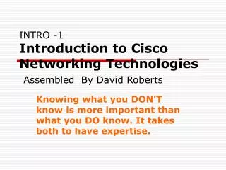
ICND -1 Interconnecting Cisco Networking Devices Assembled By David Roberts. Knowing what you DON’T know is more important than what you DO know. It takes both to have expertise. Course Content.

E N D
ICND -1 Interconnecting Cisco Networking Devices Assembled By David Roberts Knowing what you DON’T know is more important than what you DO know. It takes both to have expertise.
Course Content • This course focuses on providing the skills and knowledge necessary to install, operate, and troubleshoot a small branch office Enterprise network, including configuring a switch, a router, and connecting to a WAN and implementing network security. A Student should be able to complete configuration and implementation of a small branch office network under supervision.
Course Objectives • Describe how networks function, identifying major components, function of network components and the Open System Interconnection (OSI) reference model. • Using the host-to-host packet delivery process, describe issues related to increasing traffic on an Ethernet LAN and identify switched LAN technology solutions to Ethernet networking issues. • Describes the reasons for extending the reach of a LAN and the methods that can be used with a focus on RF wireless access. • Describes the reasons for connecting networks with routers and how routed networks transmit data through networks using TCP / IP. • Describe the function of Wide Area Networks (WANs), the major devices of WANs, and configure PPP encapsulation, static and dynamic routing, PAT and RIP routing. • Use the command-line interface to discover neighbors on the network and managing the router¿s startup and configuration .
Course Outline • Module 1 - Building a Simple Network • Module 2 - Ethernet Local Area Networks • Module 3 - Wireless Local Area Networks • Module 4 - Exploring the Functions of Routing • Module 5 - Wide Area Networks • Module 6 - Network Environment Management
Module 1 - Building a Simple Network • Connect 3 PC’s together in a Class C, Class B & Class A using IP addresses provided below. Test connectivity with ping. Class C: PC1: 10.0.0.15 /24 (255.255.255.0) PC2: 10.0.0.16 /24 (255.255.255.0) PC3: 10.0.0.17 /24 (255.255.255.0) Class B: PC1: 10.0.1.15 /16 (255.255.0.0) PC2: 10.0.2.15 /16 (255.255.0.0) PC3: 10.0.100.1 /16 (255.255.0.0) Class A: PC1: 100.200.100.100 /8 (255.0.0.0) PC2: 100.200.200.200 /8 (255.0.0.0) PC3: 100.1.2.3 /8 (255.0.0.)
Module 1 - Building a Simple Network – Part 2 • With the Class A IP’s still in place, change the subnet to a class B. Use a subnet of /16. (255.255.0.0) • What happens to the connectivity between the machines? Why? • What change to the IP address of PC3 can be made in order to restore connectivity between all three PC’s?
Module 1 - Building a Simple Network – Part 3 • Reset all PC’s to the Class C addressing scheme: • Class C: PC1: 10.0.0.15 /24 (255.255.255.0) • PC2: 10.0.0.16 /24 (255.255.255.0) • PC3: 10.0.0.17 /24 (255.255.255.0) • On PC1 bring up a command line and type in “ping –t 10.0.0.16” • On PC2 type in “ping –t 10.0.0.17” • On PC3 type in “ping –t 10.0.0.15” • Load up a packet sniffer of your choice on one of the PC’s and monitor the NIC. • Write down the MAC address for each PC that you see in the sniffer. • What port are the pings coming in & out from? • What protocol are the ping packets being sent over? • What is the actual alpha-numeric hex string that the ping packet uses as its data? This can be found in the hex information window. You may have to stop the scanner to isolate one packet. • Why cant the sniffer see all three PC’s?
Module 2 - Ethernet Local Area Networks Frames are the format of data packets on the wire. Note that a frame viewed on the actual physical hardware would show start bits, sometimes called the preamble, and the trailing Frame Check Sequence. These are required by all physical hardware and is seen in all four following frame types. They are not displayed by packet sniffing software because these bits are removed by the Ethernet adapter before being passed on to the network protocol stack software.
Module 2 - Ethernet Local Area Networks – Part 2 • Main procedure of transmission over ethernet: • Frame ready for transmission • Is medium idle? If not, wait until it becomes ready and wait the interframe gap period (9.6 µs in 10 Mbit/s Ethernet). • Start transmitting • Does a collision occur? If so, go to collision detected procedure. • Reset retransmission counters and end frame transmission • Collision detected procedure - Continue transmission until minimum packet time is reached (jam signal) to ensure that all receivers detect the collision • Increment retransmission counter • Is maximum number of transmission attempts reached? If so, abort transmission. • Calculate and wait random backoff period based on number of collisions • Re-enter main procedure at stage 1
Module 2 - Ethernet Local Area Networks – Part 3 Dual speed hubs In the early days of Fast Ethernet, Ethernet switches were relatively expensive devices. However, hubs suffered from the problem that if there were any 10BASE-T devices connected then the whole system would have to run at 10 Mbit. Therefore a compromise between a hub and a switch appeared known as a dual speed hub. These devices consisted of an internal two-port switch, dividing the 10BASE-T (10 Mbit) and 100BASE-T (100 Mbit) segments. The device would typically consist of more than two physical ports. When a network device becomes active on any of the physical ports, the device attaches it to either the 10BASE-T segment or the 100BASE-T segment, as appropriate. This prevented the need for an all-or-nothing migration from 10BASE-T to 100BASE-T networks. These devices are often known as dual-speed hubs, since the traffic between devices connected at the same speed is not switched.
Module 2 - Ethernet Local Area Networks – Part 4 • More advanced networks • Simple switched Ethernet networks, while an improvement over hub based Ethernet, suffer from a number of issues: • They suffer from single points of failure. If any link fails some devices will be unable to communicate with other devices and if the link that fails is in a central location lots of users can be cut off from the resources they require. • It is possible to trick switches or hosts into sending data to your machine even if it's not intended for it, as indicated above. • Large amounts of broadcast traffic whether malicious, accidental or simply a side effect of network size can flood slower links and/or systems. • It is possible for any host to flood the network with broadcast traffic forming a denial of service attack against any hosts that run at the same or lower speed as the attacking device. • As the network grows normal broadcast traffic takes up an ever greater amount of bandwidth. • If switches are not multicast aware multicast traffic will end up treated like broadcast traffic due to being directed at a MAC with no associated port. • If switches discover more MAC addresses than they can store (either through network size or through an attack) some addresses must inevitably be dropped and traffic to those addresses will be treated the same way as traffic to unknown addresses, that is essentially the same as broadcast traffic (this issue is known as failopen). • They suffer from bandwidth choke points where a lot of traffic is forced down a single link. • Some switches offer a variety of tools to combat these issues including: • Spanning-tree protocol to maintain the active links of the network as a tree while allowing physical loops for redundancy. • Various port protection features, as it is far more likely an attacker will be on an end system port than on a switch-switch link. • VLANs to keep different classes of users separate while using the same physical infrastructure. • fast routing at higher levels to route between those VLANs. • Link aggregation to add bandwidth to overloaded links and to provide some measure of redundancy, although the links won't protect against switch failure because they connect the same pair of switches.
Module 2 - Ethernet Local Area Networks – Part 5 • Duplex: • Terms originally referring to specific circuit designs for serial communication, but now referring more to specific rules for data flow. A simplex circuit allows only one-way communication from a transmitter to a receiver. A half-duplex circuit allows two-way communication, but only in one direction at a time; that is, the two parties to the connection must take turns transmitting and receiving data. A full-duplex circuit allows both parties to send and receive data simultaneously.
Module 2 - Ethernet Local Area Networks – Part 6 Your typical RJ-45 connector. You will find this connector most commonly on Cat-5 & Cat-6 twisted pair. The RJ-45 has 8 brass leads, 4 pairs twisted together to produce minimal distortion & signal loss on the line.
Crossover cables are used when connecting two PC’s or switches directly together. Most network equipment manufactured within the last two years has auto X-over negotiation built into the device. Module 2 - Ethernet Local Area Networks – Part 7 Console Cables are used to directly connect to management interfaces (serial port) on network equipment.
Module 2 - Ethernet Local Area Networks – Part 8 Example of unshielded twisted pair (top) & shielded twisted pair (bottom). Your basic RJ-45 tip crimp tool.
Module 2 - Ethernet Local Area Networks – Part 8-LAB • At this point take a sample of Cat-5 & tip it for crossover functionality. • Test the cable, why do the testers show an error? Is the cable good or bad? • Use the crossover to bypass the switch between two of the PC’s.
Module 3 - Wireless Local Area Networks • Wireless Encryption Types: WEP • Short for Wired Equivalent Privacy, a security protocol for wireless local area networks (WLANs) defined in the 802.11b standard. WEP is designed to provide the same level of security as that of a wired LAN. LANs are inherently more secure than WLANs because LANs are somewhat protected by the physicalities of their structure, having some or all part of the network inside a building that can be protected from unauthorized access. WLANs, which are over radio waves, do not have the same physical structure and therefore are more vulnerable to tampering. WEP aims to provide security by encrypting data over radio waves so that it is protected as it is transmitted from one end point to another. However, it has been found that WEP is not as secure as once believed. WEP is used at the two lowest layers of the OSI model - the data link and physical layers; it therefore does not offer end-to-end security. • WEP is total crap & should NEVER be used on ANY wireless network unless it is the ONLY encryption available.
Module 3 - Wireless Local Area Networks – Part 2 • Wireless Encryption Types: WPA1 • Short for Wi-Fi Protected Access, a Wi-Fistandard that was designed to improve upon the security features of WEP. The technology is designed to work with existing Wi-Fi products that have been enabled with WEP (i.e., as a software upgrade to existing hardware), but the technology includes two improvements over WEP: • Improved data encryption through the temporal key integrity protocol (TKIP). TKIP scrambles the keys using a hashingalgorithm and, by adding an integrity-checking feature, ensures that the keys haven’t been tampered with. • User authentication, which is generally missing in WEP, through the extensible authentication protocol (EAP). WEP regulates access to a wireless network based on a computer’s hardware-specific MAC address, which isrelatively simple to be sniffed out and stolen. EAP is built on a more secure public-key encryption system to ensure that only authorized network users can access the network. • It should be noted that WPA is an interim standard that will be replaced with the IEEE’s 802.11i standard upon its completion. (this was completed in 2004) • While WPA1 is very strong it can be broken with enough computing power, time & a stupid administrator who doesn’t know how to pick & choose appropriate passwords. • Using a password that includes at least one capitol, one number, one special char (~ . $ ^ #) and that is a minimum of 25 characters ensures a secure wireless network if one must use WPA1 for user compatibility.
Module 3 - Wireless Local Area Networks – Part 3 • Wireless Encryption Types: WPA2 • WPA2 implements the mandatory elements of 802.11i. In particular, in addition to TKIP and the Michael algorithm, it introduces a new AES-based algorithm, CCMP, that is considered fully secure. Note that from March 13, 2006, WPA2 certification is mandatory for all new devices wishing to be Wi-Fi certified. • Vendor support: • Official support for WPA2 in Microsoft Windows XP was rolled out on 1 May2005. Driver upgrades for network cards may be required. • Apple Computer supports WPA2 on all AirPort Extreme-enabled Macintoshes, the AirPort Extreme Base Station, and the AirPort Express. Firmware upgrades needed are included in AirPort 4.2, released July 14, 2005. • wpa_supplicant for Linux, BSD, and Windows supports WPA2 if used with a supported wireless card/driver. • WPA2 is the only wireless encryption that has not been broken. It is the strongest form of wireless security to date.
Module 3 - Wireless Local Area Networks – Part 4 • Wireless Standards: IEEE 802.11 (B) • Data Rate: Up to 11Mbps in the 2.4GHz band • Products that adhere to this standard are considered "Wi-Fi Certified." Not interoperable with 802.11a. Requires fewer access points than 802.11a for coverage of large areas. Offers high-speed access to data at up to 300 feet from base station. 14 channels available in the 2.4GHz band (only 11 of which can be used in the U.S. due to FCC regulations) with only three non-overlapping channels.
Module 3 - Wireless Local Area Networks – Part 5 • Wireless Standards: IEEE 802.11 (A) • Data Rate: Up to 54Mbps in the 5GHz band • Products that adhere to this standard are considered "Wi-Fi Certified." Eight available channels. Less potential for RF interference than 802.11b and 802.11g. Better than 802.11b at supporting multimedia voice, video and large-image applications in densely populated user environments. Relatively shorter range than 802.11b. Not interoperable with 802.11b.
Module 3 - Wireless Local Area Networks – Part 6 • Wireless Standards: IEEE 802.11 (G) • Data Rate: Up to 54Mbps in the 2.4GHz band • Products that adhere to this standard are considered "Wi-Fi Certified." May replace 802.11b. Improved security enhancements over 802.11. Compatible with 802.11b. 14 channels available in the 2.4GHz band (only 11 of which can be used in the U.S. due to FCC regulations) with only three non-overlapping channels.
Module 3 - Wireless Local Area Networks – Part 7 • Wireless Standards: 802.16 (WiMAX) • Data Rate: Variable. Specifies WiMAX in the 10 to 66 GHz range • Commonly referred to as WiMAX or less commonly as WirelessMAN or the Air Interface Standard, IEEE 802.16 is a specification for fixed broadband wireless metropolitan access networks (MANs) • 802.16a added suppor tfor the 2 to 11 GHz range.
Module 3 - Wireless Local Area Networks – Part 8 • Wireless Standards: Bluetooth • Data Rate: Up to 2Mbps in the 2.45GHz band • No native support for IP, so it does not support TCP/IP and wireless LAN applications well. Not originally created to support wireless LANs. Best suited for connecting PDAs, cell phones and PCs in short intervals. • While Bluetooth was designed for ranged of about 15 feet special “Bluetooth Sniper Rifles” can listen in on Bluetooth traffic from over a mile away if the user has a LoS (line of sight) to the source. • Bluetooth has been broken (encryption cracked), assume everything you do over it is being watched by those looking to steal your ident & bank accounts.
Module 3 - Wireless Local Area Networks – Part 9 • Wireless dangers. • AdHoc: At Starbucks it’s Christmas every day for identity thieves. It’s so easy you wouldn’t believe. • What you see to the right is all it takes to compromise the person next to you in the airport, coffee shop, library, hotel, conference, etc.. • What would happen if you had two wireless NIC’s (network interface card) in your laptop with internet sharing enabled between the two? What if you made one AdHoc and named it “Free Public Wifi”? (AdHoc wireless devices function as an AP (Access Point) & broadcast their SSID). And for the final step what do you think you could capture while monitoring that wireless NIC with a packet sniffer? • Microsoft was kind enough to have AdHoc AP’s on auto-connect anytime the SSID is seen after the first attempt. This particular “Free Public Wifi” is the most widely used SSID by thieves around the world. This SSID can be found everywhere from Africa to Europe to probably right outside your window. • Use free wifi at your own risk. You may think your smarter than your stupid neighbor who is just leaving his ‘Linksys’ wireless unsecured, but he may be much, much smarter than you… capturing every username & password of every credit card, bank account & personal sites you log into.
Module 3 - Wireless Local Area Networks – Part 9-LAB • Wireless Lab: • Reset wireless router to default. • Set administrative password. • Set SSID & de-activate SSID broadcast. • Set encryption to WPA1 & choose a 25 character key. • Set up a client & connect to the wireless router. • Sniff the traffic.
Module 4 – Exploring the Functions of Routing • Before we get into the details of routing protocols & path determination algorithms lets first examine the diagram to the right to get a good understanding of what routing is used for. • Take note of the different networks & their placement. • 10.1.128.0, 10.1.130.0 & 10.1.129.0 are the networks that make up the backbone. • 10.1.2.0, 10.1.3.0 & 10.1.1.0 are the networks that make up the distribution layers. • While this diagram does not specify what the subnet is, we can assume that they are all Class C subnets of /24, (255.255.255.0) • If Daffy sends a packet addressed for Elmer it will hit Albuquerque first. If Albuquerque does not know that the network 10.1.3.0 exists it will drop the packet. If the router has been configured to forward packets destined for anything in the range 10.1.3.0 to Seville it will do so. • Routers at the most basic functionality are merely traffic directors that point down one road or the other depending on where the traffic wants to go. They do this by keeping a massive roadmap that is either programmed by an administrator manually or discovered automatically by a routing protocol. • In this diagram you see that a packet coming from Daffy destined for Elmer can go out either s0 or s1. Different routing protocols have different algorithms that determine which route to take. This is called Path Cost Analysis.
Module 4 – Exploring the Functions of Routing – Part 2 • Routing fundamentals: • There are 3 basic rules that you can keep in mind while you learn that will help keep new concepts clear. • A router never needs to “route” a packet destined for a network range it is directly connected to. • No two interfaces on a router can be assigned an IP address in the same network. • A router may have MANY different IP addresses assigned to a single interface. It is not at all uncommon for a packet to go into an interface on one network and go right back out again the same interface on a different network.
Module 4 – Exploring the Functions of Routing – Part 3 • Routing Protocol Fundamentals: Distance Vector Routing • A distance-vector routing protocol is one of the two major classes of routing protocols used in packet-switched networks for computer communications, the other major class being the link-state protocol. A distance-vector routing protocol uses the Bellman-Ford algorithm to calculate paths. • Examples of distance-vector routing protocols include RIPv1 or 2 and IGRP. EGP and BGP are not pure distance-vector routing protocols but their concepts are the same. In many cases, EGP and BGP are considered DV (distance-vector) routing protocols. • A distance-vector routing protocol requires that a router informs its neighbors of topology changes periodically and, in some cases, when a change is detected in the topology of a network. Compared to link-state protocols, which requires a router to inform all the nodes in a network of topology changes, distance-vector routing protocols have less computational complexity and message overhead.
Module 4 – Exploring the Functions of Routing – Part 4 • Routing Protocol Fundamentals: Link-state routing • A link-state routing protocol is one of the two main classes of routing protocols used in packet-switched networks for computer communications. Examples of link-state routing protocols include OSPF and IS-IS. • The link-state protocol is performed by every switching node in the network (i.e. nodes which are prepared to forward packets; in the Internet, these are called routers). The basic concept of link-state routing is that every node receives a map of the connectivity of the network, in the form of a graph showing which nodes are connected to which other nodes. • Each node then independently calculates the best next hop from it for every possible destination in the network. (It does this using only its local copy of the map, and without communicating in any other way with any other node.) The collection of best next hops forms the routing table for the node. • This contrasts with distance-vector routing protocols, which work by having each node share its routing table with its neighbors. In a link-state protocol, the only information passed between the nodes is information used to construct the connectivity maps.
Module 4 – Exploring the Functions of Routing – Part 5 • Routing Protocols: RIPv1 & RIPv2 • The Routing Information Protocol (RIP) is one of the most commonly used interior gateway protocol (IGP) routing protocols on internal networks (and to a lesser extent, networks connected to the Internet), which helps routers dynamically adapt to changes of network connections by communicating information about which networks each router can reach and how far away those networks are. • Although RIP is still actively used, it is generally considered to have been made obsolete by routing protocols such as OSPF and IS-IS. Nonetheless, a somewhat more capable protocol in the same basic family (distance-vector routing protocols), was Cisco's proprietary (IGRP) Interior Gateway Routing Protocol. Cisco does not support IGRP in current releases of its software. It was "replaced" by EIGRP, the Enhanced Interior Gateway Routing Protocol, which is a completely new design. While EIGRP is still technically distance vector, it relates to IGRP only in having a similar name. • RIP is sometimes said to stand for Rest in Pieces in reference to the reputation that RIP has for breaking unexpectedly, rendering a network unable to function.
Module 4 – Exploring the Functions of Routing – Part 6 • Routing Protocols: RIP Continued • RIP is a distance-vector routing protocol, which employs the hop count as a routing metric. The maximum number of hops allowed with RIP is 15, and the hold down time is 180 seconds. Originally each RIP router transmits full updates every 30 seconds by default. Originally, routing tables were small enough that the traffic was not significant. • As networks grew in size, however, it became evident there could be a massive burst every 30 seconds, even if the routers had been initialized at random times. It was thought, as a result of random initialization, the routing updates would spread out in time, but this was not true in practice. Sally Floyd and Van Jacobson published research in 1994 [1] that showed having all routers use a fixed 30 second timer was a very bad idea. Without slight randomization of the update timer, this research showed that the timers weakly synchronized over time and sent their updates out at the same time. Modern RIP implementations introduce deliberate time variation into the update timer of each router. • It runs at the network layer of the Internet protocol suite. RIP prevents routing loops from continuing indefinitely by implementing a limit on the number of hops allowed in a path from the source to a destination. This hop limit, however, limits the size of networks that RIP can support. • RIP implements the split horizon and holddown mechanisms to prevent incorrect routing information from being propagated. These are some of the stability features of RIP. • In many current networking environments RIP would not be the first choice for routing as its convergence times and scalability are poor compared to EIGRP, OSPF, or IS-IS (the latter two being link-state routing protocols), and the hop limit severely limits the size of network it can be used in. On the other hand, it is easier to configure because, using minimal settings for any routing protocols, RIP does not require any parameter on a router whereas all the other protocols require at least one or more parameters
Module 4 – Exploring the Functions of Routing – Part 7 • Routing Protocols: RIP Continued.1 • RIPv1: defined in RFC 1058, uses classful routing. The routing updates do not carry subnet information, lacking support for variable length subnet masks (VLSM). This limitation makes it impossible to have different-sized subnets inside of the same network class. In other words, all subnets in a network class must be the same size. There is also no support for router authentication, making RIPv1 slightly vulnerable to various attacks. • RIPv2: Due to the above deficiencies of RIPv1, RIPv2 was developed in 1994 and included the ability to carry subnet information, thus supporting Classless Inter-Domain Routing (CIDR). However to maintain backwards compatibility the 15 hop count limit remained. Rudimentary plain text authentication was added to secure routing updates; later, MD5 authentication was defined in RFC 2082. Also, in an effort to avoid waking up hosts that do not participate in the routing protocol, RIPv2 multicasts routing updates to 224.0.0.9, as opposed to RIPv1 which uses broadcast.
Module 4 – Exploring the Functions of Routing – Part 7-LAB • At this time please complete Sequential Labs # 1-6 & Stand Alone Labs # 12. This Requires Boson Cisco CCNA Network Simulator. Chapter reading is included with the software. • Read the Chapters • Read the Chapters • Read the Chapters
Module 4 – Exploring the Functions of Routing – Part 8 • Routing Concepts: Split horizon • In computer networks, distance-vector routing protocols employ the split horizon rule which prohibits a router from advertising a route back out the interface from which it was learned. Split horizon is one of the methods used to prevent routing loops due to the slow convergence times of distance-vector routing protocols. • In this example A uses the path via B to reach C. A will not advertise its route for C back to B. On the surface, this seems redundant since B will never use A's route because it costs more than B's route to C. However, if B's route to C goes down, B could end up using A's route, which goes through B; A would send the packet right back to B, creating a loop. With split horizon, this particular loop scenario cannot happen. An additional variation of split horizon does advertise the route back to the router that is used to reach the destination, but marks the advertisement as unreachable. This is called split horizon with poison reverse.
Module 4 – Exploring the Functions of Routing – Part 9 • Routing Protocols: IGRP • Interior Gateway Routing Protocol (IGRP) is a kind of IGP which is a distance-vector routing protocol invented by Cisco, used by routers to exchange routing data within an autonomous system. • IGRP was created in part to overcome the limitations of RIP (maximum hop count of only 15, and a single routing metric) when used within large networks. IGRP supports multiple metrics for each route, including bandwidth, delay, load, MTU, and reliability; to compare two routes these metrics are combined together into a single metric, using a formula which can be adjusted through the use of pre-set constants. The maximum hop count of IGRP-routed packets is 255 (default 100). • IGRP is considered a classful routing protocol. As the protocol has no field for a subnet mask the router assumes that all interface addresses have the same subnet mask as the router itself. This contrasts with classless routing protocols that can use variable length subnet masks. Classful protocols have become less popular as they are wasteful of IP address space. • In order to address the issues of address space and other factors, Cisco created EIGRP (Enhanced Interior Gateway Routing Protocol). EIGRP adds support for VLSM (variable length subnet mask) and adds the Diffusing Update Algorithm (DUAL) in order to improve routing and provide a loopless environment. EIGRP has completely replaced IGRP, making IGRP an obsolete routing protocol. In Cisco IOS versions 12.3 and greater, IGRP is completely unsupported. IGRP is still taught in Cisco's CCNA curriculum, but it should be noted that knowledge of IGRP is not tested.
Module 4 – Exploring the Functions of Routing – Part 15 • Routing Concepts: Route Summarization • Route summarization, also know as route aggregation, summarizes a group of routes into a single route advertisement. Route summarization can be used as a powerful tool in a networking environment. The demand for increased network capabilities has resulted from corporate expansions and mergers. The number of subnets and network addresses contained in routing table is rapidly increasing based on these expansions. This growth has had a negative impact on CPU resources, bandwidth, and memory used to maintain the routing tables. Therefore, route summarization was introduced as a way to reduce the size of network routing tables. • If configured properly, route summarization can reduce the latency associated with router hop, since the average speed for routing table lookup will be increased due to the reduced number of entries. The overhead for routing protocols can also be reduced since fewer routing entries are being advertised. • Another advantage of using route summarization in large, complex networks is that it can isolate topology changes from other routers. This can aid in improving the stability of the network by limiting the propagation of routing traffic after a network link goes down. For example, if a router only advertises a summary route to the next router hop, then it will not advertise any changes to specific subnets within the summarized range. This can significantly reduce any unnecessary routing updates following a topology change. Hence, increasing the speed of convergence and allowing for a more stable environment.
Module 4 – Exploring the Functions of Routing – Part 16 • Routing Concepts: Route Summarization Continued • As an example of how summarization can be used as a powerful tool in a networking environment imagine a company that operates 150 accounting services in each of the 50 states and each accounting office has a router and frame relay link connected to its corporate office. Without route summarization, the routing table on any given router would have to maintain 150 routers times 50 states = 7,500 different networks. However, if route summarization is implemented, then each state would have a centralized site to connect it with all other offices. Since each router is summarized before being advertised to other states, then every router will only see its own subnets and 49 summarized entries representing other states. This would create less stress on the router’s CPU, memory, and bandwidth.
Module 4 – Exploring the Functions of Routing – Part 17 • Routing Concepts: Route Summarization Continued.1 • In order to determine the summary route on a router, you must first decide the number of highest-order bits that match in all addresses. See the following example which shows the process of calculating a summary route. • In the table below, Router A has the following networks in its routing table: • 192.168.98.0192.168.99.0192.168.100.0192.168.101.0192.168.102.0192.168.105.0 • First of all, you must convert the addresses to binary format and align them in a list as shown in the table to the right. Second, locate the bits where the common pattern of digits ends (those in red). Lastly, count the number of common bits. The summary route number is represented by the first IP address in the block, followed by a slash, followed by the number of common bits. Summarized route is 192.168.96.0/20 As you can see, the first 20 bits of the IP address are the same. Hence, the best summary route can be advertised as 192.168.96.0/20. For summarization to work properly, multiple IP addresses must share the same highest-order bits and should only be implemented within classless routing protocols such as EIGRP, OSPF, RIP v.2, IS-IS for IP, and BGP. In some cases, this feature may not be feasible. For example, in RIP v.1 is a classful routing protocol that automatically summarizes based on class when advertising across a major network boundary. Automatic route summarization can potentially cause problems if summarization occurs at more than one point in the network since the summarized routes may be in conflict. When this occurs, a router receives identical summary routes from different directions. This can lead to serious connectivity issues.
Module 5 – Wide Area Networks • The great Google has collected these definitions of a WAN: • A network of computers spread out across a great distance. WANs are often networks of networks, linking local area networks into a single network.faculty.tamu-commerce.edu/espinoza/s/carpenter-p/cl1.html • (WANs) are networks that generally span distances greater than one city and include regional networks such as telephone companies or international networks such as global communications services providers.www.wiley.co.uk/college/turban/glossary.html • A wide area network or WAN is a computer network covering a wide geographical area, involving vast array of computers. This is different from personal area networks (PANs), metropolitan area networks (MANs) or local area networks (LANs) that are usually limited to a room, building or campus. The best example of a WAN is the Internet. en.wikipedia.org/wiki/Wide_area_networks
Module 5 – Wide Area Networks – Part 4 • PPP Encapsulation • PPP (Point-to-Point Protocol) is a protocol for communication between two computers using a serial interface, typically a personal computer connected by phone line to a server. For example, your Internet server provider may provide you with a PPP connection so that the provider’s server can respond to your requets, pass them on to the Internet, and forward your requested Internet responses back to you. PPP uses the Internet Protocol (IP) (and is designed to handle other). It is sometimes considered a member of the TCP/IP suite of protocols. Relative to the Open Systems Interconnection (OSI) reference model, PPP provides layer 2 (data-link layer) service. Essentially, it packages your computer’s TCP/IP packets and forwards them to the server where they can actually be put on the Internet. • PPP is a full-duplex protocol that can be used on various physical media, including twisted pair or fiber optic lines or satellite transmission. It uses a variation of High Speed Data Link Control (HDLC) for packet encapsulation. • PPP is usually preferred over the earlier de facto standard Serial Line Internet Protocol (SLIP) because it can handle synchronous as well as asynchronous communication. PPP can share a line with other users and it has error detection that SLIP lacks. Where a choice is possible, PPP is prefered.
Module 5 – Wide Area Networks – Part 4-LAB • At this point do Stand Alone Labs # 16 , Scenario Labs # 10 & Sequential Lab # 15. • These labs cover PPP encapsulation & NAT/PAT routing. • READ CHAPTER 8 & 9