Download
1 / 63
630 likes | 647 Views
This article explores data structures and programming techniques for implementing dynamic sets and disjoint sets. It covers topics such as representing finite, dynamic sets, implementing dynamic sets using various data structures, constructing sets, finding elements in sets, uniting sets, determining connected components in undirected graphs, computing minimum spanning trees, and maintaining equivalence relations.

E N D
Data Structures for Disjoint Sets ManolisKoubarakis Data Structures and Programming Techniques
Dynamic Sets • Sets are fundamental for mathematics but also for computer science. • In computer science, we usually study dynamic sets i.e., sets that can grow, shrink or otherwise change over time. • The data structures we have presented so far in this course offer us ways to represent finite, dynamic sets and manipulate them on a computer. Data Structures and Programming Techniques
Dynamic Sets and Symbol Tables • Many of the data structures we have so far presented for symbol tables can be used to implement a dynamic set (e.g., a linked list, a hash table, a (2,4) tree etc.). Data Structures and Programming Techniques
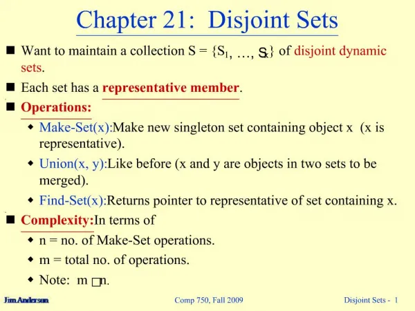
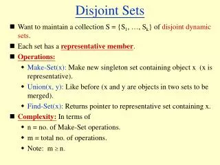
Disjoint Sets • Some applications involve grouping distinct elements into a collection of disjoint sets(ξένα σύνολα). • Important operations in this case are to construct a set, to find which set a given element belongs to, and to unite two sets. Data Structures and Programming Techniques
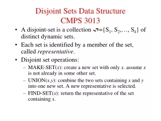
Definitions • A disjoint-set data structure maintains a collection of disjoint dynamic sets. • Each set is identified by a representative (αντιπρόσωπο), which is some member of the set. • The disjoint sets might form a partition (διαμέριση) of a universe set Data Structures and Programming Techniques
Definitions (cont’d) • The disjoint-set data structure supports the following operations: • Make-Set(): It creates a new set whose only member (and thus representative) is pointed to by . Since the sets are disjoint, we require that not already be in any of the existing sets. • Union(): It unites the dynamic sets that contain and , say and , into a new set that is the union of these two sets. One of the and give its name to the new set and the other set is “destroyed” by removing it from the collection . The two sets are assumed to be disjoint prior to the operation. The representative of the resulting set is some member of (usually the representative of the set that gave its name to the union). • Find-Set() returns a pointer to the representative of the unique set containing . Data Structures and Programming Techniques
Determining the Connected Components of an Undirected Graph • One of the many applications of disjoint-set data structures is determining the connected components (συνεκτικές συνιστώσες) of an undirected graph. • The implementation based on disjoint-sets that we will present here is appropriate when the edges of the graph are not static e.g., when edges are added dynamically and we need to maintain the connected components as each edge is added. Data Structures and Programming Techniques
Example Graph h a b e f j i c g d Data Structures and Programming Techniques
Computing the Connected Components of an Undirected Graph • The following procedure Connected-Components uses the disjoint-set operations to compute the connected components of a graph. Connected-Components() for each vertex doMake-Set( for each edge do if Find-Set()Find-Set() thenUnion() Data Structures and Programming Techniques
Computing the Connected Components (cont’d) • Once Connected-Components has been run as a preprocessing step, the procedure Same-Component given below answers queries about whether two vertices are in the same connected component. Same-Component() if Find-Set()Find-Set() then return TRUE else return FALSE Data Structures and Programming Techniques
Example Graph h a b e f j i c g d Data Structures and Programming Techniques
The Collection of Disjoint Sets After Each Edge is Processed Data Structures and Programming Techniques
Minimum Spanning Trees • Another application of the disjoint set operations that we will see is Kruskal’s algorithm for computing the minimum spanning tree of a graph. Data Structures and Programming Techniques
Maintaining Equivalence Relations • Another application of disjoint-set data structures is to maintain equivalence relations. • Definition. An equivalence relation on a set is relation with the following properties: • Reflexivity: for all , we have . • Symmetry: for all , if then . • Transitivity: for all , if and then . Data Structures and Programming Techniques
Examples of Equivalence Relations • Equality • Equivalent type definitions in programming languages. For example, consider the following type definitions in C: struct A { int a; int b; }; typedef A B; typedef A C; typedef A D; • The types A, B, C and D are equivalent in the sense that variables of one type can be assigned to variables of the other types without requiring any casting. Data Structures and Programming Techniques
Equivalent Classes • If a set has an equivalence relation defined on it, then the set can be partitioned into disjoint subsets called equivalence classes whose union is • Each subset consists of equivalent members of . That is, for all and in , and if and are in different subsets. Data Structures and Programming Techniques
Example • Let us consider the set . • The equivalence relation on is defined by the following: • Note that the relation follows from the others given the definition of an equivalence relation. Data Structures and Programming Techniques
The Equivalence Problem • The equivalence problem can be formulated as follows. • We are given a set and a sequence of statements of the form • We are to process the statements in order in such a way that, at any time, we are able to determine in which equivalence class a given element of belongs. Data Structures and Programming Techniques
The Equivalence Problem (cont’d) • We can solve the equivalence problem by starting with each element in a named set. • When we process a statement , we call Find-Set() and Find-Set(). • If these two calls return different sets then we call Union to unite these sets. If they return the same set then this statement follows from the other statements and can be discarded. Data Structures and Programming Techniques
Example (cont’d) • We start with each element of in a set: • As the given equivalence relations are processed, these sets are modified as follows: 3 follows from the other statements and is discarded Data Structures and Programming Techniques
Example (cont’d) • Therefore, the equivalent classes of are the subsets and . Data Structures and Programming Techniques
Linked-List Representation of Disjoint Sets • A simple way to implement a disjoint-set data structure is to represent each set by a linked list. • The first object in each linked list serves as its set’s representative. The remaining objects can appear in the list in any order. • Each object in the linked list contains a set member, a pointer to the object containing the next set member, and a pointer back to the representative. Data Structures and Programming Techniques
The Structure of Each List Object Set Member Pointer to Next Object Pointer Back to Representative Data Structures and Programming Techniques
Example: the Sets {c, h, e, b} and {f, g, d} . c b e h . f d g The representatives of the two sets are c and f. Data Structures and Programming Techniques
Implementation of Make-Set and Find-Set • With the linked-list representation, both Make-Set and Find-Set are easy. • To carry out Make-Set(), we create a new linked list which has one object with set element • To carry out, Find-Set(), we just return the pointer from back to the representative. Data Structures and Programming Techniques
Implementation of Union • To perform Union(), we can append ’s list onto the end of ’s list. • The representative of the new set is the element that was originally the representative of the set containing • We should also update the pointer to the representative for each object originally in ’s list. Data Structures and Programming Techniques
Amortized Analysis • In an amortized analysis (επιμερισμένη ανάλυση), the time required to perform a sequence of data structure operations is averaged over all operations performed. • Amortized analysis can be used to show that the average cost of an operation is small, if one averages over a sequence of operations, even though a single operation might be expensive. • Amortized analysis differs from the average-case analysis in that probability is not involved; an amortized analysis guarantees the average performance of each operation in the worst case. Data Structures and Programming Techniques
Techniques for Amortized Analysis • The aggregate method(η μέθοδος της συνάθροισης). With this method, we show that for all , a sequence of operations takes time in total, in the worst case. Therefore, in the worst case, the average cost, or amortized cost, per operation is • The accounting method. • The potential method. • We will only use the aggregate method in this lecture. For the other methods, see any advanced algorithms book e.g., the one cited in the readings. Data Structures and Programming Techniques
Complexity Parameters for the Disjoint-Set Data Structures • We will analyze the running time of our data structures in terms of two parameters: • , the number of Make-Set operations, and • , the total number of Make-Set, Union and Find-Set operations. • Since the sets are disjoint, each union operation reduces the number of sets by one. Therefore, after Union operations, only one set remains. The number of Union operations is thus at most . • Since the Make-Set operations are included in the total number of operations, we have . Data Structures and Programming Techniques
Complexity of Operations for the Linked List Representation • Make-Set and Find-Set take time. • Union( takes time where and denote the cardinalities of the sets that contain and . We need time to reach the last object in ’s list to make it point to the first object in ’s list. We also need time to update all pointers to the representative in ’s list. • If we keep a pointer to the last object in the list in each representative then we do not need to scan ’s list, and we only need time to update all pointers to the representative in ’s list. • In both cases, the complexity of Union is since the cardinality of each set can be at most . Data Structures and Programming Techniques
Complexity (cont’d) • We can prove that there is a sequence of Make-Set and Union operations that take time. Therefore, the amortized time of an operation is . • Proof? Data Structures and Programming Techniques
Proof • Let and • Suppose that we have objects • We then execute the sequence of operations shown on the next slide. Data Structures and Programming Techniques
Operations Data Structures and Programming Techniques
Proof (cont’d) • We spend time performing the Make-Set operations. • Because the -thUnion operation updates objects, the total number of objects updated are . • The total time spent therefore is which is since and Data Structures and Programming Techniques
The Weighted Union Heuristic • The above implementation of the Union operation requires an average of time per operation because we may be appending a longer list onto a shorter list, and we must update the pointer to the representative of each member of the longer list. • If each representative also includes the length of the list then we can always append the smaller list onto the longer, with ties broken arbitrarily. This is called the weighted union heuristic. Data Structures and Programming Techniques
Theorem • Using the linked list representation of disjoint sets and the weighted union heuristic, a sequence of Make-Set, Union and Find-Set operations, of which are Make-Set operations, takes time. • Proof? Data Structures and Programming Techniques
Proof • We start by computing, for each object in a set of size , an upper bound on the number of times the object’s pointer back to the representative has been updated. • Consider a fixed object We know that each time ’s representative pointer was updated, must have started in the smaller set and ended up in a set (the union) at least twice the size of its own set. • For example, the first time ’s representative pointer was updated, the resulting set must have had at least 2 members. Similarly, the next time ’s representative pointer was updated, the resulting set must have had at least 4 members. • Continuing on, we observe that for any , after ’s representative pointer has been updated times, the resulting set must have at least members. • Since the largest set has at most members, each object’s representative pointer has been updated at most times over all Union operations. The total time used in updating objects is thus . Data Structures and Programming Techniques
Proof (cont’d) • The time for the entire sequence of operations follows easily. • Each Make-Set and Find-Set operation takes time, and there are of them. • The total time for the entire sequence is thus . Data Structures and Programming Techniques
Complexity (cont’d) • The bound we have just shown can be seen to be , therefore the amortized time for each of the operations is • There is a faster implementation of disjoint sets which improves this amortized complexity. • We will present this method now. Data Structures and Programming Techniques
Disjoint-Set Forests • In the faster implementation of disjoint sets, we represent sets by rooted trees. • Each node of a tree represents one set member and each tree represents a set. • In a tree, each set member points only to its parent. The root of each tree contains the representative of the set and is its own parent. • For many sets, we have a disjoint-set forest. Data Structures and Programming Techniques
Example: the Sets {b, c, e, h} and{d, f, g} c f d h e g b The representatives of the two sets are c and f. Data Structures and Programming Techniques
Implementing Make-Set,Find-Set and Union • A Make-Set operation simply creates a tree with just one node. • A Find-Set operation can be implemented by chasing parent pointers until we find the root of the tree. The nodes visited on this path towards the root constitute the find-path. • A Union operation can be implemented by making the root of one tree to point to the root of the other. Data Structures and Programming Techniques
Example: the Union of Sets {b, c, e, h} and {d, f, g} f c d h e g b Data Structures and Programming Techniques
Complexity • With the previous data structure, we do not improve on the linked-list implementation. • A sequence of Union operations may create a tree that is just a linear chain of nodes. Then, a Find-Set operation can take time. Similarly, for a Union operation. • By using the following two heuristics, we can achieve a running time that is almost linear in the number of operations . Data Structures and Programming Techniques
The Union by Rank Heuristic • The first heuristic, union by rank, is similar to the weighted union heuristic we used with the linked list representation. • The idea is to make the root of the tree with fewer nodes to point to the root of the tree with more nodes. • We will not explicitly keep track of the size of the subtree rooted at each node. Instead, for each node, we maintain a rank that approximates the logarithm of the size of the subtree rooted at the node and is also an upper bound on the height of the node (i.e., the number of edges in the longest path between and a descendant leaf). • In union by rank, the root with the smaller rank is made to point to the root with the larger rank during a Union operation. Data Structures and Programming Techniques
The Path Compression Heuristic • The second heuristic, path compression, is also simple and very effective. • This heuristic is used during Find-Set operations to make each node on the find path point directly to the root. • In this way, trees with small height are constructed. • Path compression does not change any ranks. Data Structures and Programming Techniques
The Path Compression Heuristic Graphically f e d c b Data Structures and Programming Techniques
The Path Compression Heuristic Graphically (cont’d) f e c b d Data Structures and Programming Techniques
Implementing Disjoint-Set Forests • With each node , we maintain the integer value rank[], which is an upper bound on the height of . • When a singleton set is created by Make-Set, the initial rank of the single node in the corresponding tree is 0. • Each Find-Set operation leaves ranks unchanged. • When applying Union to two trees, we make the root of higher rank the parent of the root of lower rank. In this case ranks remain the same. In case of a tie, we arbitrarily choose one of the roots as the parent and increment its rank. Data Structures and Programming Techniques
Pseudocode We designate the parent of node by p[]. Make-Set() p[]← rank[] ← 0 Union() Link(Find-Set(), Find-Set()) Data Structures and Programming Techniques